Introduction
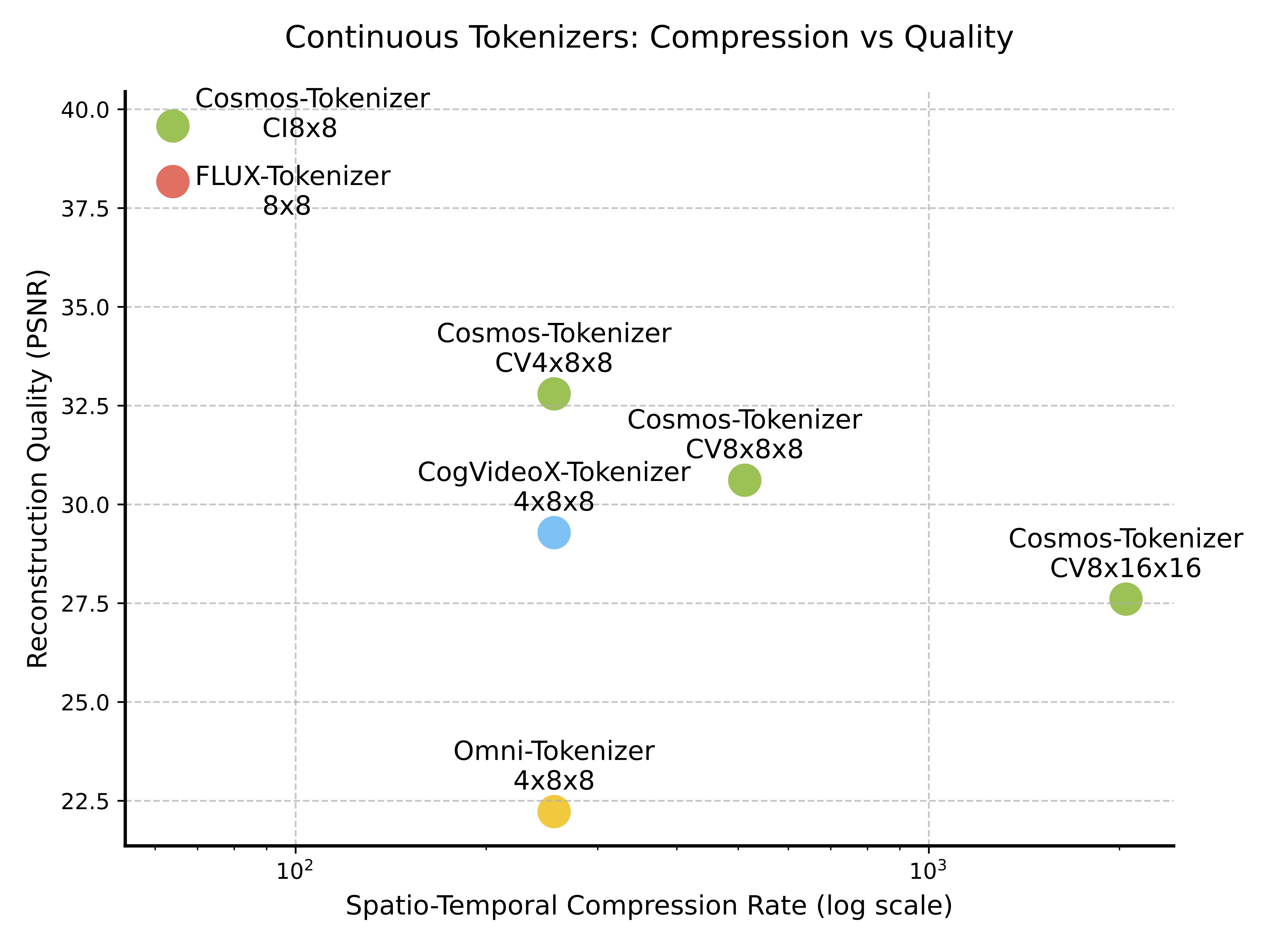
(a) Continuous tokenizers
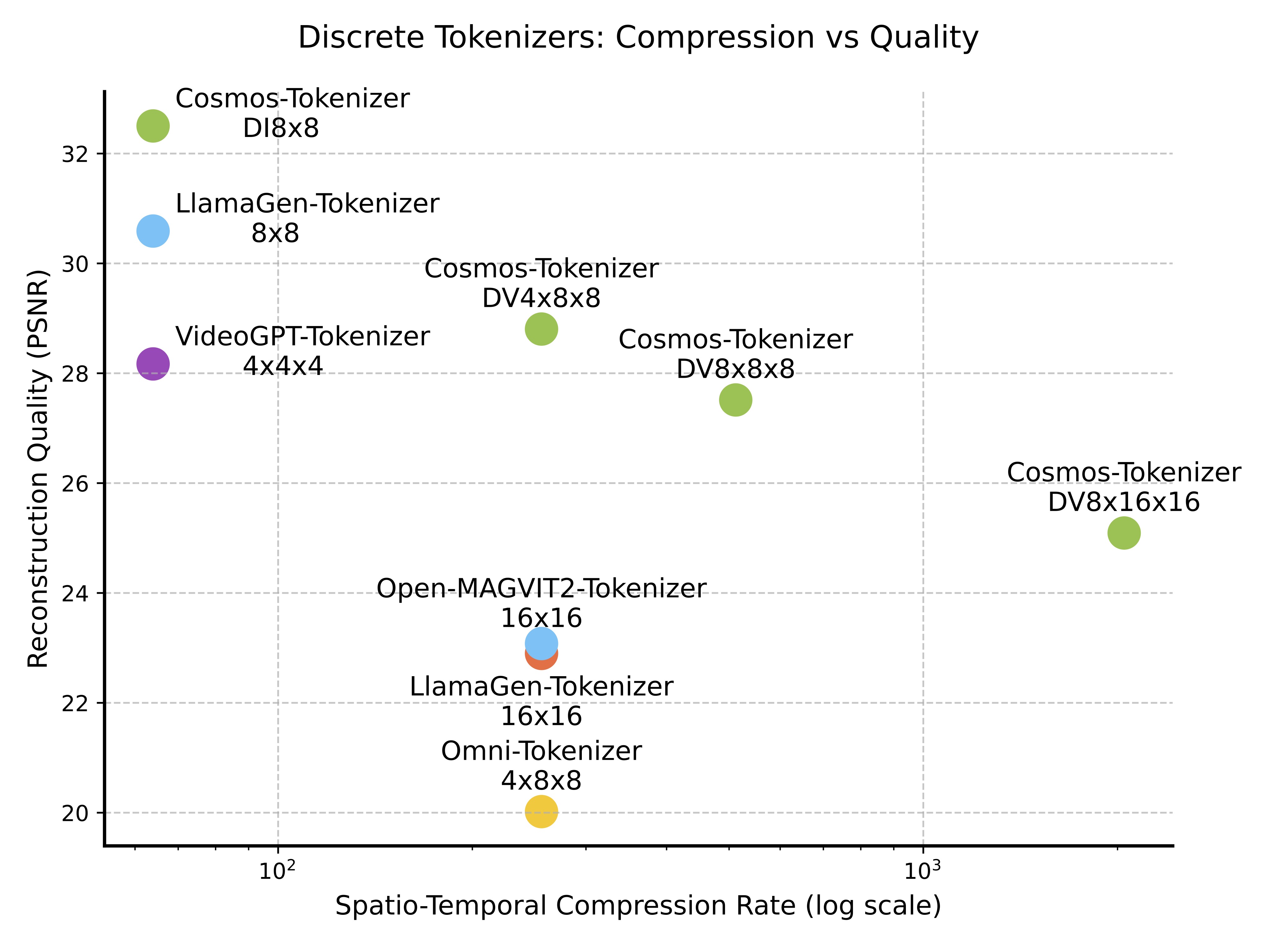
(b) Discrete tokenizers
Figure 1: Comparison of continuous (left) and discrete (right) tokenizers on spatio-temporal compression rate (log scale) vs. reconstruction quality (PSNR). Each point shows a tokenizer configuration's compression-quality trade-off. Our tokenizer achieves superior quality even at higher compression rates compared to other methods.
Tokenizers are key components in generative AI, converting raw data into efficient, compressed representations by discovering latent spaces through unsupervised learning. Visual tokenizers specifically transform high-dimensional visual data, like images and videos, into compact semantic tokens, enabling efficient large-scale model training and reducing computational demands for inference. Figure 2 illustrates a tokenization pipeline for videos.
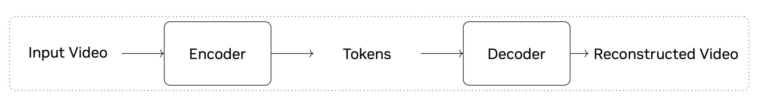
Figure 2: Video tokenization pipeline. An input video is encoded into tokens, which are usually much more compact than the input video. The decoder then reconstructs the input video from the tokens. Tokenizer training is about learning the encoder and decoder to preserve the visual information in the tokens maximally.
There are two types of tokenizers: continuous and discrete. Continuous tokenizers map visual data to continuous embeddings, suitable for models sampling from continuous distributions, such as Stable Diffusion (Rombach et al., 2022). Discrete tokenizers map visual data to quantized indices, used in models like VideoPoet (Kondratyuk et al., 2024) that rely on cross-entropy loss for training, like the GPT models. Figure 3 compares these token types.
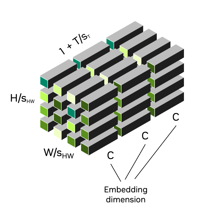
(a) Continuous tokenizers
(b) Discrete tokenizers
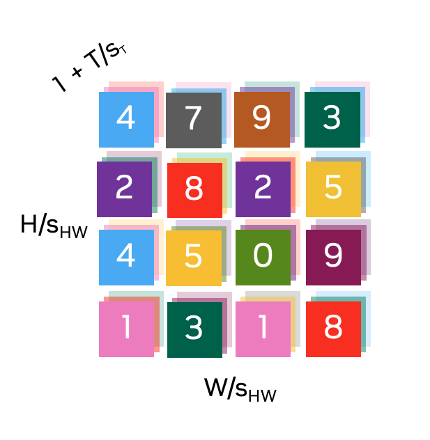
Figure 3: Tokens along spatial (\(\frac{H}{s_{HW}} \times \frac{W}{s_{HW}}\)) and temporal (\(1+\frac{T}{s_{T}}\)) dimensions, with a spatial compression factor of \(s_{HW}\) and a temporal compression factor of \(s_{T}\). The first temporal token represents the first input frame, enabling joint image (\(T=0\)) and video (\(T>0\)) tokenization in a shared latent space. (a) Continuous latent embeddings with an embedding size of \(C\), and (b) Quantized indices, each color representing a discrete latent code.
Tokenizers must balance high compression with quality, preserving visual details in the latent space. We introduce Cosmos Tokenizer, a comprehensive suite of continuous and discrete visual tokenizers for images and videos that delivers remarkable compression, high-quality reconstruction, and speeds up to 12X faster than previous methods. It supports various image and video types, with flexible compression rates to accommodate diverse computational constraints, as shown in Table 1.
| Models | Causal | Image | Video | Joint | Discrete | Continuous |
|---|---|---|---|---|---|---|
| FLUX (FLUX, 2024) | — | ✓ | ✗ | ✗ | ✗ | ✓ |
| Open-MAGVIT2 (Luo et al., 2024) | — | ✓ | ✗ | ✗ | ✓ | ✗ |
| LlamaGen (Sun et al., 2024) | — | ✓ | ✗ | ✗ | ✓ | ✗ |
| VideoGPT (Yan et al., 2021) | ✗ | ✗ | ✓ | ✗ | ✓ | ✗ |
| Omni (Wang et al., 2024) | ✗ | ✓ | ✓ | ✓ | ✓ | ✓ |
| CogX-VAE (Yang et al., 2024) | ✓ | ✓ | ✓ | ✓ | ✗ | ✓ |
| Cosmos (Ours) | ✓ | ✓ | ✓ | ✓ | ✓ | ✓ |
Cosmos Tokenizer is built on a lightweight, temporally causal architecture, using causal temporal convolution and attention layers to maintain the order of video frames. This unified design allows seamless tokenization for both images and videos.
We train Cosmos Tokenizer on high-resolution images and long videos, covering a wide range of aspect ratios (including 1:1, 3:4, 4:3, 9:16, and 16:9) across diverse categories of data. During inference, it is agnostic to temporal length, allowing it to tokenize beyond its training length.
We evaluated Cosmos Tokenizer on standard datasets, including MS-COCO 2017, ImageNet-1K, FFHQ, CelebA-HQ, and DAVIS. To standardize video tokenizer evaluation, we also curated a new dataset, called TokenBench, covering categories like robotics, driving, and sports, which we have made publicly available at github.com/NVlabs/TokenBench. Results (Figure 1) show Cosmos Tokenizer significantly outperforms existing methods, with a +4 dB PSNR gain on DAVIS videos. It tokenizes up to 12× faster and can encode up to 8-second 1080p and 10-second 720p videos on NVIDIA A100 GPUs with 80GB memory. Pretrained models, with spatial compressions of 8× and 16× and temporal compressions of 4× and 8×, are available at github.com/NVIDIA/Cosmos-Tokenizer.
Architecture
The Cosmos Tokenizer is designed as an encoder-decoder architecture. Given an input video \(x_{0:T} \in \mathbb{R}^{(1+T) \times H \times W \times 3}\) with height \(H\), width \(W\), and frames \(T\), the encoder (\(\mathcal{E}\)) compresses it into tokens \(z_{0:T'} \in \mathbb{R}^{(1+T') \times H' \times W' \times C}\) with spatial and temporal compression factors \(s_{HW}\) and \(s_T\), respectively. The decoder (\(\mathcal{D}\)) reconstructs the video as \(x'_{0:T} \in \mathbb{R}^{(1+T) \times H \times W \times 3}\), mathematically as:
\[x'_{0:T} = \mathcal{D}\Big(\mathcal{E}\big(x_{0:T}\big)\Big).\]
Our architecture employs a temporally causal design, processing only current and past frames at each stage. The tokenizer operates in the wavelet transform space, where a 2-level wavelet transform downsamples inputs by a factor of four, grouping frames as \(\{g_0, g_1, \dots\} = \{x_0, x_{1:4}, x_{5:8}, \dots\}\). Subsequent stages encode these groups causally, ultimately outputting tokens \(z_{0:T'}\). This causal design is essential for physical AI applications, which often operate in a similar causal setting, and the wavelet transform enables effective compression by emphasizing semantic content.
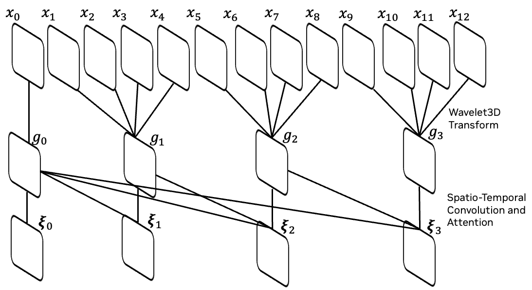
(a) Temporal Causality: Illustration of the temporal causality mechanism, where inputs \(x_0, x_1, \dots, x_{12}\) are processed through grouped intermediate outputs via wavelet transform \(g_0, g_1, \dots\), and further refined by causal spatio-temporal convolution and attention operations.
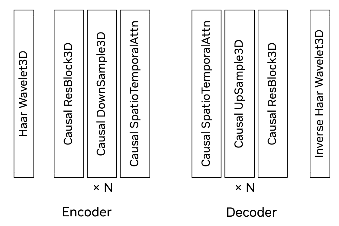
(b) Network Architecture: The encoder-decoder network structure includes a 3D Haar wavelet, causal residual, downsampling, and spatio-temporal attention blocks. The decoder mirrors the encoder's structure.
Figure 4: Cosmos Tokenizer architecture.
Our encoder stages (after the wavelet transform) consist of residual blocks interleaved with down-sampling blocks. Each encoder block applies a spatio-temporal factorized 3D convolution: a 2D convolution of \(1 \times k \times k\) captures spatial information, followed by a temporal convolution of \(k \times 1 \times 1\) to capture dynamics, with left padding of \(k-1\) ensuring causality. Long-range dependencies are captured through a spatio-temporal factorized causal self-attention with a global support region, e.g., \(1+T'\) in the last encoder block. The decoder mirrors the encoder but replaces downsampling with upsampling. Figure 4 shows the Cosmos Tokenizer architecture.
We use a vanilla autoencoder (AE) to model continuous tokenizers' latent space and Finite-Scalar-Quantization (FSQ) (Mentzer et al., 2023) for discrete tokenizers. The latent dimension for continuous tokenizers is 16, while for discrete tokenizers it is 6, with FSQ levels of (8, 8, 8, 5, 5, 5), resulting in a vocabulary size of 64,000.
Training
We use a joint training strategy, alternating mini-batches of images and videos at a preset frequency. We supervise only the final output of the tokenizer's decoder, without auxiliary losses in the latent spaces (e.g., commitment or KL prior losses). For instance, a VAE for continuous tokenizers would require a KL prior loss, and a VQ-VAE for discrete quantization would require a commitment loss, unlike our vanilla AE and FSQ approach.
We employ a two-stage training scheme. In the first stage, we optimize with the L1 loss that minimizes the pixel-wise RGB difference between the input and reconstructed video (\(\hat{x}_{0:T}\)), given by \[\mathcal{L}_1 = \left\lVert \hat{x}_{0:T} - x_{0:T} \right\rVert_1,\] and the perceptual loss based on the VGG-19 features (Simonyan and Zisserman, 2014), given by, \[\mathcal{L}_{\text{Perceptual}} = \frac{1}{L} \sum_{l=1}^{L} \sum_{t} \alpha_l \left\lVert \texttt{VGG}_l (\hat{x}_t) - \texttt{VGG}_l (x_t) \right\rVert_1,\] where \(\texttt{VGG}_l (\cdot) \in \mathbb{R}^{H \times W \times C}\) is the features from the \(l\)-th layer of a pre-trained VGG-19 network, \(L\) is the number of layers considered, and \(\alpha_{l}\) is the weight of the \(l\)-th layer. When \(x\) is a video (i.e. \(T>0\)), we compute the perceptual loss as the average of the per-frame perceptual losses.
In the second stage, we use the optical flow (\(\texttt{OF}\)) loss (Teed and Deng, 2020) to handle the temporal smoothness of reconstructed videos, \[\mathcal{L}_{\text{Flow}} = \frac{1}{T} \sum_{t=2}^{T+1} \left\lVert \texttt{OF}(\hat{x}_{t}, \hat{x}_{t-1}) - \texttt{OF}(x_{t}, x_{t-1}) \right\rVert_1 + \frac{1}{T} \sum_{t=1}^{T} \left\lVert \texttt{OF}(\hat{x}_{t}, \hat{x}_{t+1}) - \texttt{OF}(x_{t}, x_{t+1}) \right\rVert_1,\] and the Gram-matrix (\(\texttt{GM}\)) loss (Gatys et al., 2016) to enhance the sharpness of reconstructed images, \[\mathcal{L}_{\text{Gram}} = \frac{1}{L} \sum_{l=1}^{L} \sum_t \alpha_l \left\lVert \texttt{GM}_l (\hat{x}_t) - \texttt{GM}_l (x_t) \right\rVert_1.\]
Additionally, we use adversarial loss in the fine-tuning stage to further enhance reconstruction details, particularly at large compression rates.
Evaluation
We extensively evaluated our Cosmos Tokenizer suite on diverse image and video benchmark datasets. For image tokenizers, we followed previous work and evaluated on MS-COCO 2017 (Lin et al., 2015), ImageNet-1K (Deng et al., 2009), FFHQ (Karras et al., 2019), and CelebA-HQ (Karras, 2017).
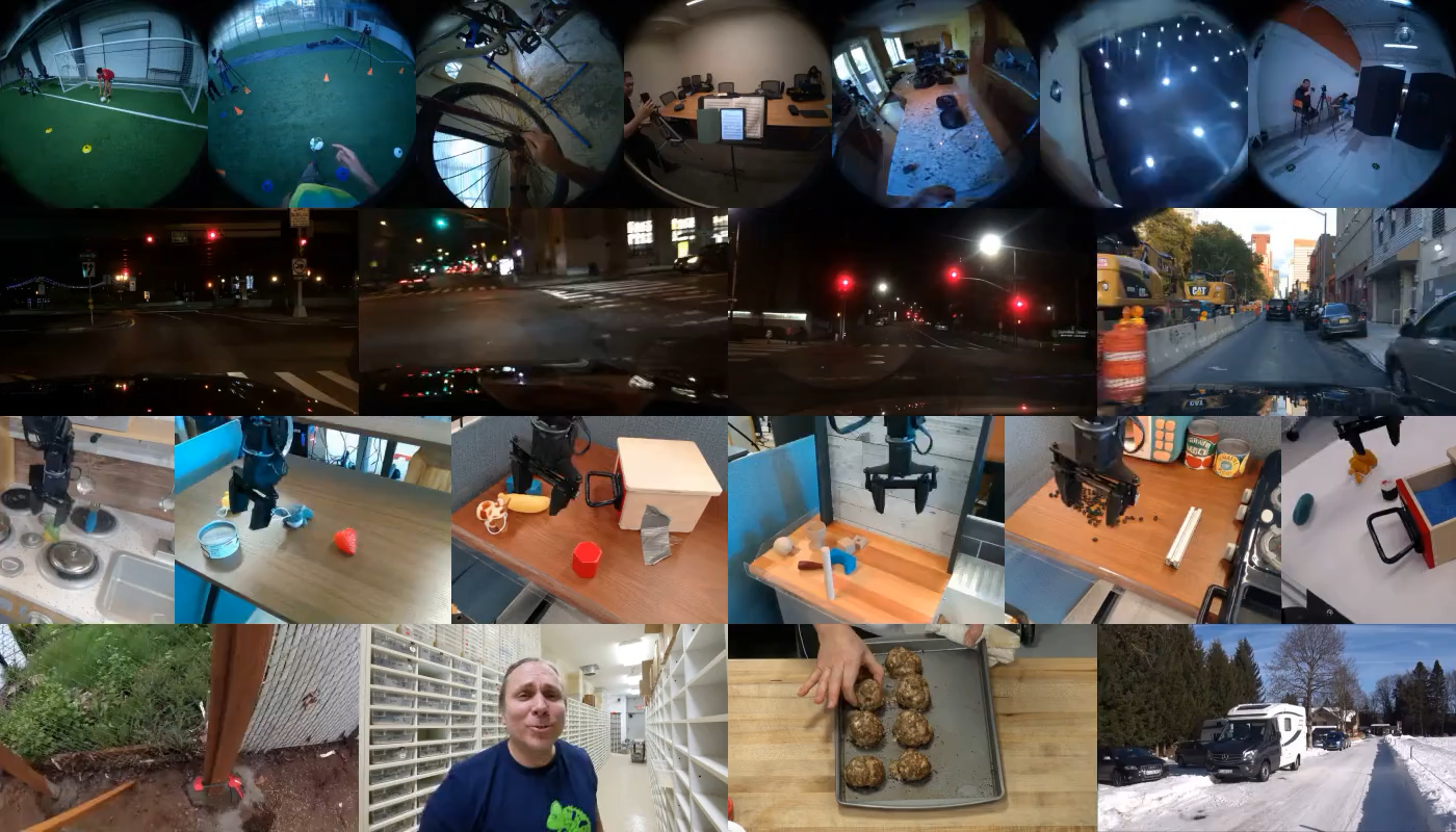
Figure 5: Example videos from TokenBench, including egocentric, driving, robotic manipulation, and web videos.
TokenBench To address the lack of standardized benchmarks for high-resolution, long-duration videos, we introduced TokenBench, covering various domains such as robotics, driving, egocentric, and web videos. TokenBench includes 100 randomly sampled, 10-second clips from each of BDD100K (Yu et al., 2020), EgoExo-4D (Grauman et al., 2024) BridgeData V2 (Walke et al., 2023), and Panda-70M (Chen et al., 2024). We manually filtered low-quality videos in Panda-70M and selected 100 scenes from EgoExo-4D, with one egocentric and one exocentric video per scene, totaling 500 videos. Examples of TokenBench are shown in Figure 5, and we have made it publicly available for the community at github.com/NVlabs/TokenBench. We also evaluated our video tokenizers on the DAVIS (Perazzi et al., 2016) dataset at 1080p.
Baselines and Evaluation Metrics We evaluated our tokenizers across different compression rates, comparing them with state-of-the-art (SOTA) image and video tokenizers (see Table 1 for details). The evaluation metrics include PSNR, SSIM, reconstruction Fréchet Inception Distance (rFID) for images, and Fréchet Video Distance (rFVD) for videos.
Qualitative Results
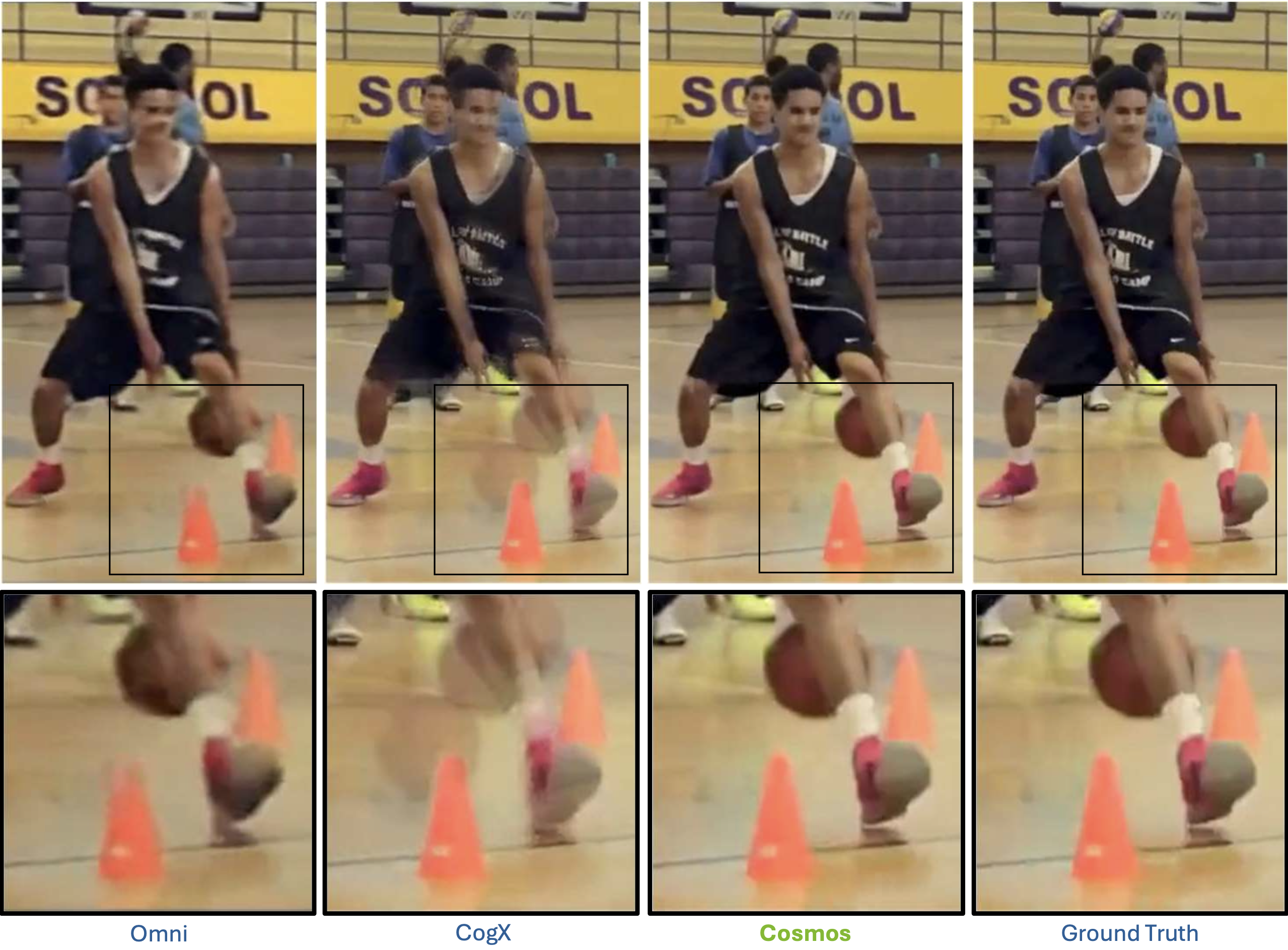
Figure 6: Comparison of video reconstruction with continuous video tokenizer with 4×8×8 compression (CV4×8×8).
Figure 6 and 7 show the reconstructed video frames using continuous video tokenizers, covering diverse scenarios such as natural scenes, autonomous driving, robotic manipulation, and egocentric videos. Figure 9 shows reconstructed images with different discrete image tokenizers, while Figure 8 presents error maps for continuous image tokenizers to highlight reconstruction differences. Compared to previous methods, Cosmos Tokenizer more effectively preserves structural and high-frequency details (e.g., grass, tree branches, text) with minimal visual distortion (e.g., faces, text) and ghosting.
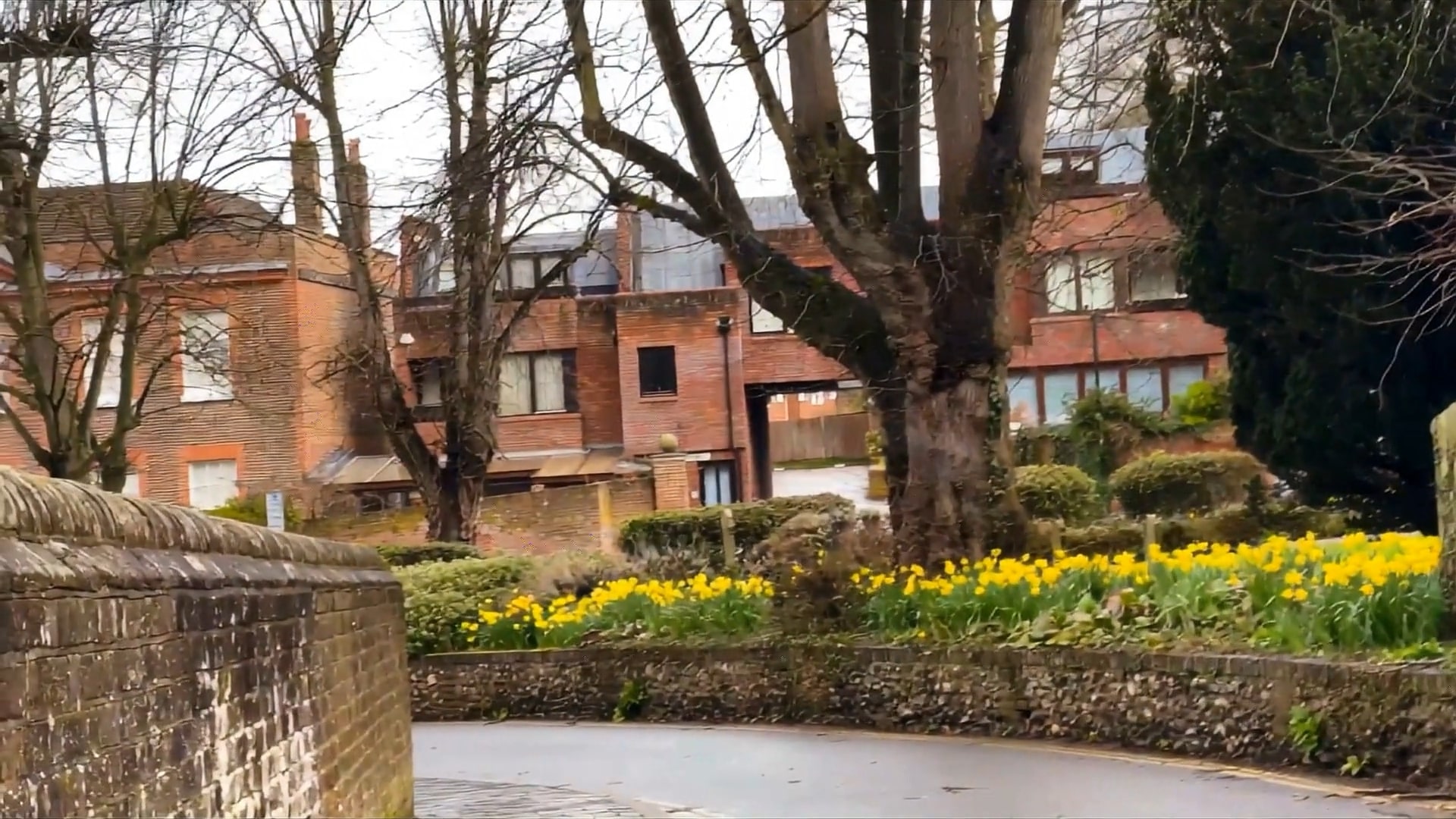
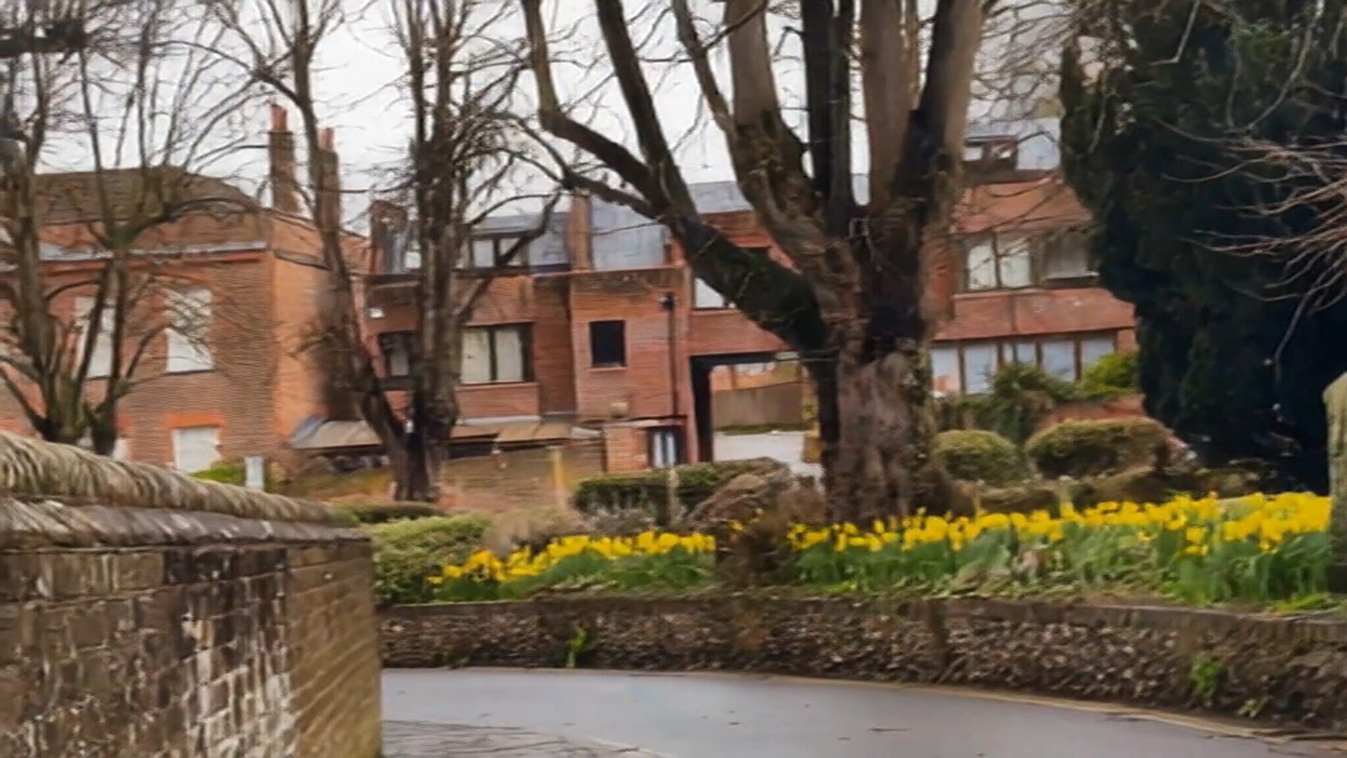
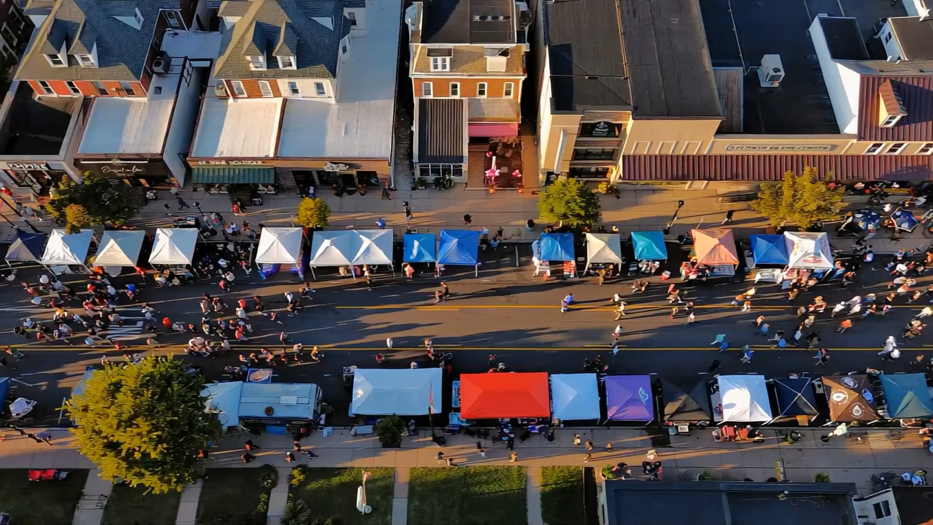


Figure 7: Comparison of video reconstruction with discrete video tokenizers with 4×8×8 compression (DV4×8×8).
These qualitative results show that Cosmos Tokenizer is capable of encoding and decoding a wide range of visual contents and has the capability to preserve the highest visual quality of images and videos.
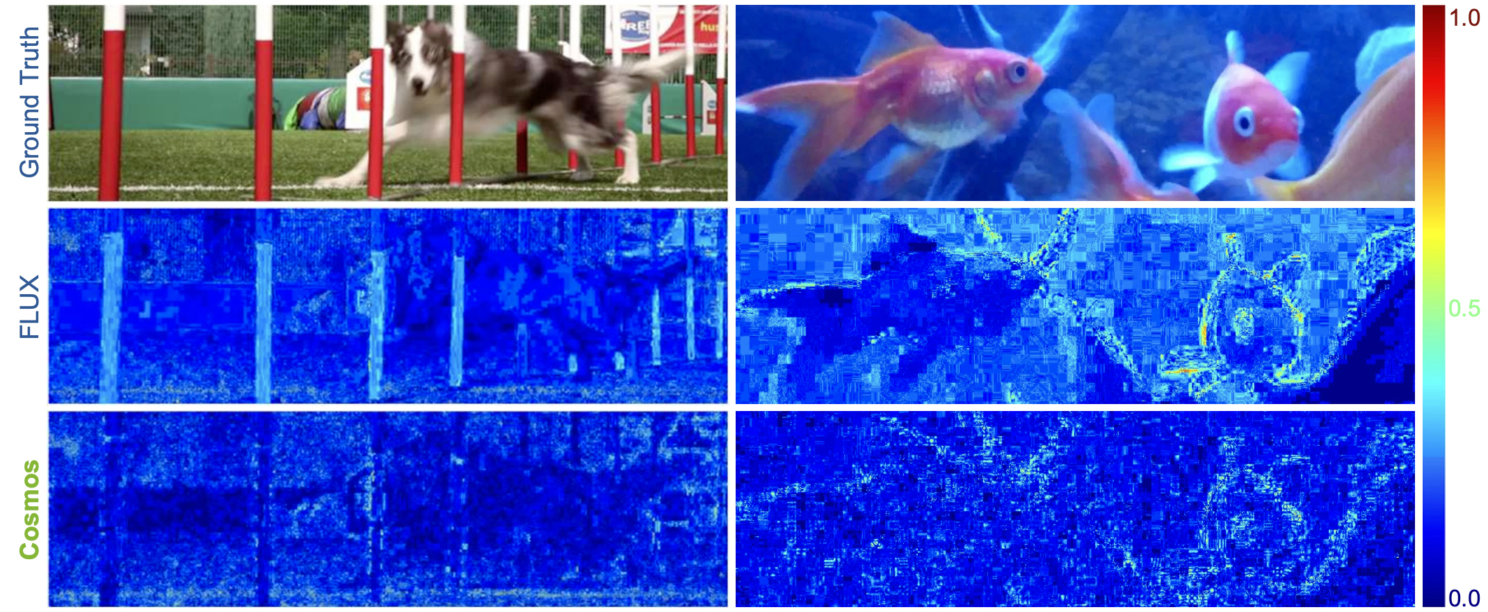
Figure 8: Comparison of image reconstruction error maps with continuous image tokenizers with 8×8 compression (CI8×8).
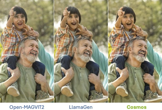
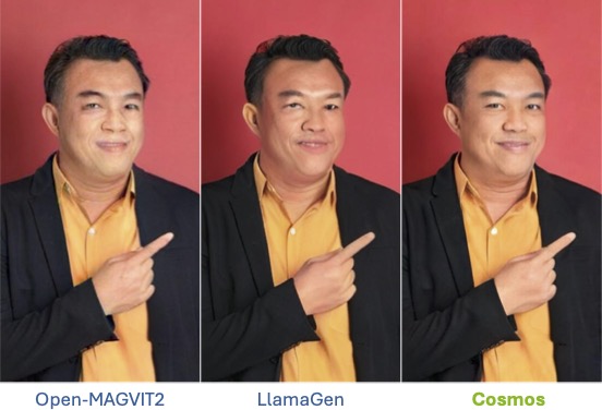
Figure 9: Comparison of image reconstruction with discrete image tokenizers with 16×16 compression (DI16×16).
Quantitative Results
Tables 2 and 3 present average quantitative metrics for continuous and discrete video tokenizers on various benchmarks. Cosmos Tokenizer achieves state-of-the-art performance on both the DAVIS and TokenBench datasets at a 4×8×8 compression ratio. Even at higher compression rates (8×8×8 and 8×16×16), Cosmos Tokenizer outperforms previous methods, demonstrating an excellent compression-quality trade-off.
| Tokenizer | Compression Ratio | Formulation | DAVIS | TokenBench | ||||
|---|---|---|---|---|---|---|---|---|
| PSNR | SSIM | rFVD | PSNR | SSIM | rFVD | |||
| CogVideoX | 4 × 8 × 8 | VAE | 29.29 | 0.864 | 19.5800 | 32.06 | 0.909 | 6.9700 |
| Omnitokenizer | 4 × 8 × 8 | VAE | 22.23 | 0.713 | 117.6600 | 24.48 | 0.830 | 35.8600 |
| Cosmos-CV | 4 × 8 × 8 | AE | 32.80 | 0.900 | 15.9300 | 35.45 | 0.928 | 6.8490 |
| Cosmos-CV | 8 × 8 × 8 | AE | 30.61 | 0.856 | 30.1600 | 34.44 | 0.917 | 11.6200 |
| Cosmos-CV | 8 × 16 × 16 | AE | 27.60 | 0.779 | 93.8200 | 31.61 | 0.875 | 43.0800 |
| Tokenizer | Compression Ratio | Quantization | DAVIS | TokenBench | ||||
|---|---|---|---|---|---|---|---|---|
| PSNR | SSIM | rFVD | PSNR | SSIM | rFVD | |||
| VideoGPT | 4 × 4 × 4 | VQ | 28.17 | 0.850 | 72.3300 | 33.66 | 0.914 | 13.8500 |
| Omnitokenizer | 4 × 8 × 8 | VQ | 20.02 | 0.703 | 188.6000 | 25.31 | 0.827 | 53.5500 |
| Cosmos-DV | 4 × 8 × 8 | FSQ | 28.81 | 0.818 | 37.3600 | 31.97 | 0.888 | 19.6700 |
| Cosmos-DV | 8 × 8 × 8 | FSQ | 27.51 | 0.789 | 100.1500 | 30.95 | 0.873 | 43.8600 |
| Cosmos-DV | 8 × 16 × 16 | FSQ | 25.09 | 0.714 | 241.5200 | 28.91 | 0.829 | 113.4800 |
Similarly, Tables 4 and 5 show that Cosmos Tokenizer consistently achieves superior results on various image benchmarks at 8×8 compression rate. Notably, at 4× larger compression rate of 16×16, the image quality of Cosmos Tokenizer often matches or surpasses prior art at 8×8. These results confirm Cosmos Tokenizer's capability to represent visual content effectively with high spatio-temporal compression.
| Tokenizer | Compression Ratio | Formulation | (a) MS-COCO 2017 | (b) ImageNet-1K | ||||
|---|---|---|---|---|---|---|---|---|
| PSNR | SSIM | rFID | PSNR | SSIM | rFID | |||
| FLUX | 8 × 8 | VAE | 24.01 | 0.692 | 2.5007 | 20.09 | 0.518 | 1.2293 |
| Cosmos-CI | 8 × 8 | AE | 28.66 | 0.836 | 1.7601 | 28.83 | 0.837 | 0.6890 |
| Cosmos-CI | 16 × 16 | AE | 23.63 | 0.663 | 3.8229 | 23.72 | 0.655 | 1.0307 |
| (c) FFHQ | (d) CelebA-HQ | |||||||
| FLUX | 8 × 8 | VAE | 38.14 | 0.960 | 0.0428 | 41.01 | 0.987 | 0.0401 |
| Cosmos-CI | 8 × 8 | AE | 39.10 | 0.957 | 0.0421 | 46.26 | 0.988 | 0.0158 |
| Cosmos-CI | 16 × 16 | AE | 30.84 | 0.829 | 0.5035 | 33.84 | 0.905 | 0.3818 |
| Tokenizer | Compression Ratio | Quantization | (a) MS-COCO 2017 | (b) ImageNet-1K | ||||
|---|---|---|---|---|---|---|---|---|
| PSNR | SSIM | rFID | PSNR | SSIM | rFID | |||
| Open-MAGVIT2 | 16 × 16 | LFQ | 19.50 | 0.502 | 6.6488 | 17.00 | 0.398 | 2.7005 |
| LlamaGen | 8 × 8 | VQ | 21.99 | 0.617 | 4.1231 | 19.64 | 0.498 | 1.4034 |
| LlamaGen | 16 × 16 | VQ | 19.11 | 0.491 | 6.0767 | 18.38 | 0.448 | 1.6573 |
| Cosmos-DI | 8 × 8 | FSQ | 24.40 | 0.704 | 3.7102 | 24.48 | 0.701 | 1.2647 |
| Cosmos-DI | 16 × 16 | FSQ | 20.45 | 0.529 | 7.2338 | 20.49 | 0.518 | 2.5178 |
| (c) FFHQ | (d) CelebA-HQ | |||||||
| Open-MAGVIT2 | 16 × 16 | LFQ | 28.20 | 0.774 | 1.9943 | 29.46 | 0.844 | 2.8649 |
| LlamaGen | 8 × 8 | VQ | 31.24 | 0.868 | 0.7011 | 33.39 | 0.936 | 0.5020 |
| LlamaGen | 16 × 16 | VQ | 27.70 | 0.772 | 1.3656 | 28.86 | 0.837 | 1.1128 |
| Cosmos-DI | 8 × 8 | FSQ | 32.50 | 0.875 | 0.4588 | 35.55 | 0.939 | 0.2647 |
| Cosmos-DI | 16 × 16 | FSQ | 27.60 | 0.750 | 1.9813 | 28.91 | 0.808 | 1.6911 |
Extended Visual Results
To further demonstrate the effectiveness of Cosmos Tokenizer, we provide comparison videos across driving, robotics, and sport videos. Pause the videos at desired temporal locations to closely inspect image quality differences.
Runtime Performance
Table 6 compares the parameters and average encoding and decoding times per image or video frame on a single A100 80GB GPU. Cosmos Tokenizer achieves 2× to 12× faster speeds than prior state-of-the-art tokenizers while maintaining the smallest model size, demonstrating high efficiency in encoding and decoding visual content.
Together with the qualitative results, quantitative metric evaluations, and the efficiency evaluation, these results demonstrate that Cosmos Tokenizer is well placed to serve as an effective and efficient building block in both diffusion-based and autoregressive models for image and video generation and the development of a world model. You can try out Cosmos Tokenizer on your projects using the source code and pre-trained models, which are now publicly available.
| Tokenizer | Type | Resolution | Compression Ratio | Parameters | Time (ms) |
|---|---|---|---|---|---|
| FLUX | Continuous-Image | 1024×1024 | 8 × 8 | 84M | 242.0 |
| Cosmos-CI | Continuous-Image | 1024×1024 | 8 × 8 | 77M | 52.7 |
| LlamaGen | Discrete-Image | 1024×1024 | 8 × 8 | 70M | 475.0 |
| Cosmos-DI | Discrete-Image | 1024×1024 | 8 × 8 | 79M | 64.2 |
| CogVideoX | Continuous-Video | 720×1280 | 4 × 8 × 8 | 216M | 414.0 |
| OmniTokenizer | Continuous-Video | 720×1280 | 4 × 8 × 8 | 54M | 82.9 |
| Cosmos-CV | Continuous-Video | 720×1280 | 4 × 8 × 8 | 105M | 34.8 |
| OmniTokenizer | Discrete-Video | 720×1280 | 4 × 8 × 8 | 54M | 53.2 |
| Cosmos-DV | Discrete-Video | 720×1280 | 4 × 8 × 8 | 105M | 51.5 |
Contributors
Fitsum Reda, Jinwei Gu, Xian Liu, Songwei Ge, Ting-Chun Wang, Haoxiang Wang, Ming-Yu Liu
Citation
Please cite as NVIDIA et al. using the following BibTex:
@article{nvidia2025cosmostokenizer,
  title={Cosmos Tokenizer: A Suite of Image and Video Neural Tokenizers},
  author={NVIDIA and Reda, Fitsum and Gu, Jinwei and Liu, Xian and Ge, Songwei and Wang, Ting-Chun and Wang, Haoxiang and Liu, Ming-Yu},
  journal={arXiv preprint arXiv:2501.03575},
  year={2025}
}