TL;DR. We propose CARV, a compute-aware variance-reduction framework for diffusion-teacher gradients, which gives a 2 to 3 times effective compute multiplier on diffusion-guided optimization and data attribution without changing the objective.
Abstract
Pretrained diffusion models serve as frozen teachers feeding downstream pipelines such as 3D generation, single-step distillation, and data attribution. The teacher gradients these pipelines consume are Monte Carlo expectations over noise levels and Gaussian noise samples; their estimator variance dominates compute cost because each draw requires expensive upstream work (rendering, simulation, encoding). We introduce CARV, a compute-aware variance-accounting framework that motivates a hierarchical Monte Carlo estimator: amortize the expensive upstream computation over cheap diffusion-noise resamples, sharpened by timestep importance sampling and a stratified inverse-CDF construction. In 3D generation and attribution experiments, CARV delivers 2 to 3 times effective compute multipliers (most from amortized reuse, with about 25% additional from importance sampling and stratification) without changing the objective. In single-step distillation, the same techniques cut gradient variance by an order of magnitude but do not improve downstream FID, indicating that MC variance is no longer the bottleneck in that setting.
Same per-step compute with sharper text-to-3D.
Both columns run at the same per-step compute: standard SDS on the left, CARV on the right.
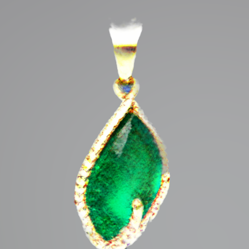
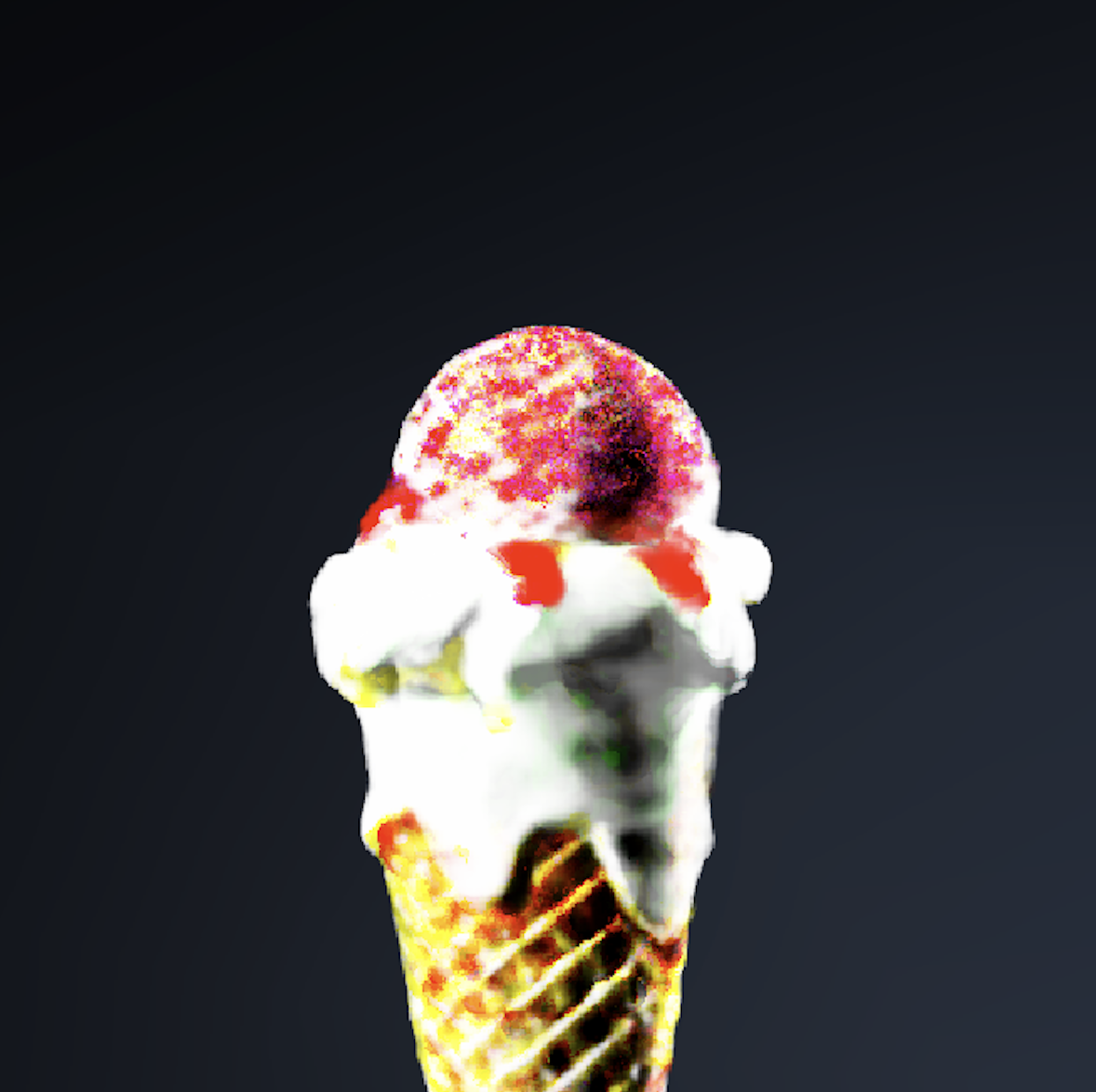
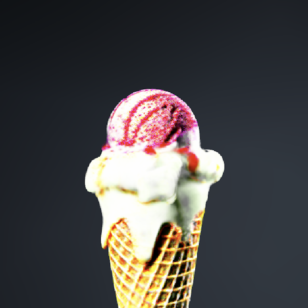
“A castle-shaped sandcastle”
Baseline
CARV
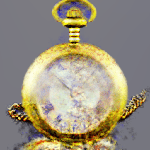
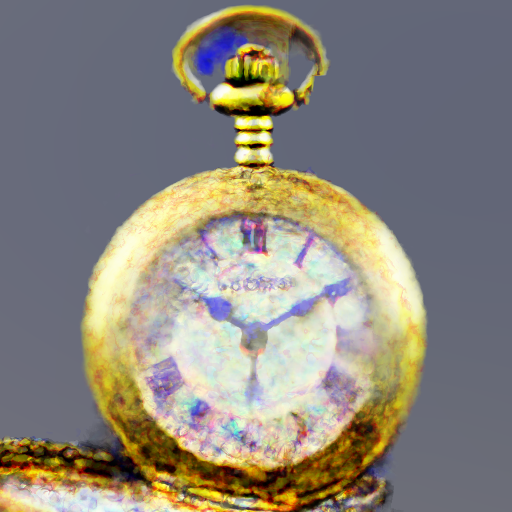
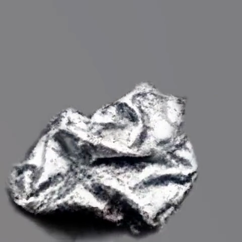
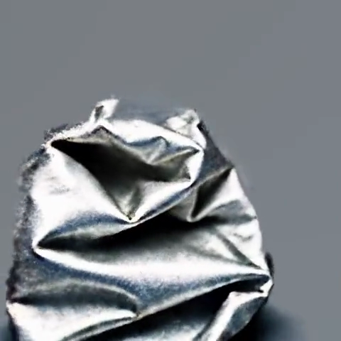
“A crumpled soda can”
Baseline
CARV
Why MC variance dominates compute
Teacher-guided pipelines all look the same on paper: form a stochastic gradient estimate, take a step, repeat. But the expensive part is rarely the diffusion model. It is the upstream render, encode, or simulate that runs before the diffusion teacher sees a sample.
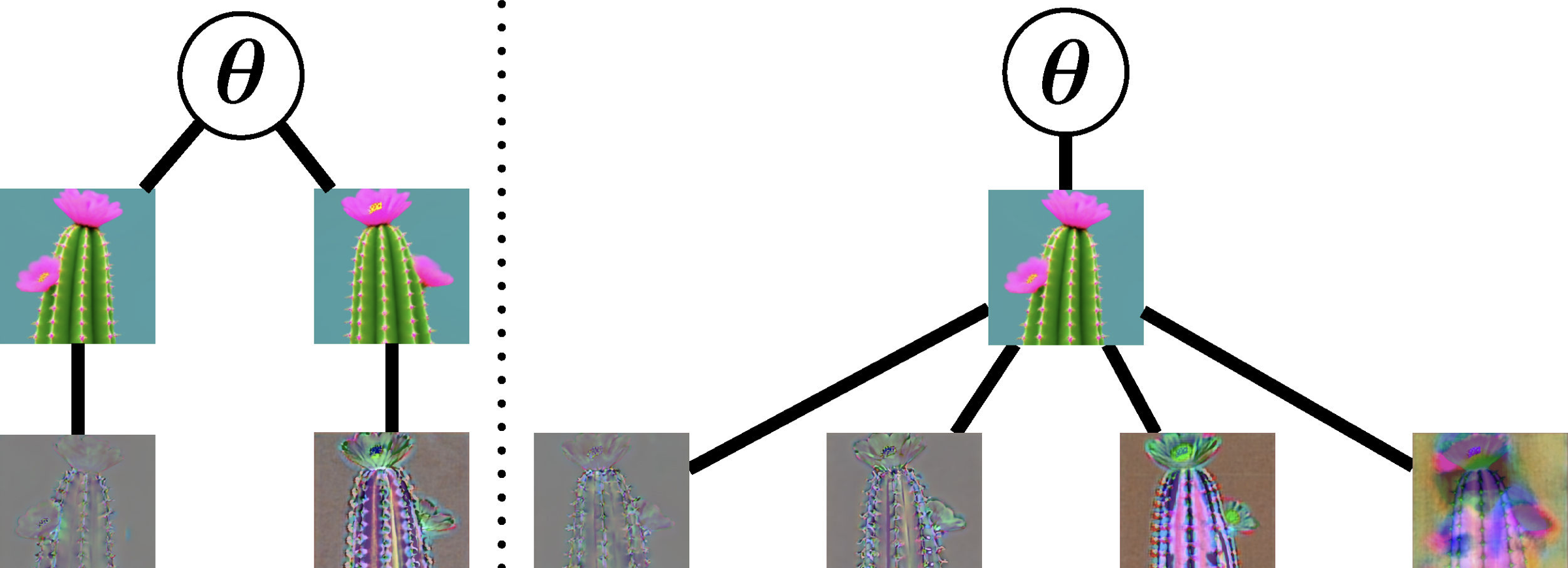
One render, many noise samples
SDS renders a 3D scene, encodes it, then asks the teacher for a denoising direction. Render and encode are the bottleneck; noising and denoising are cheap. So we make the cheap part work harder: resample $(t, \epsilon)$ many times per render, reuse the encoded latent.
Variance, not bias, sets the budget
Most pipelines inherit a timestep distribution, average more samples, and tune compute blindly. CARV measures gradient variance against compute and tells you which axis to attack: timestep allocation, noise resamples, or render reuse.
Method: three drop-in fixes
All three fixes are unbiased under the stated sampling, replace a few lines of the per-step sampling logic, and stack on top of any SDS, DMD, or TRAK pipeline that already calls a diffusion teacher.
1. Amortized compute reuse: the largest contribution
Hold the expensive render and encode fixed and resample the cheap diffusion noise. Cache the latent of one render and pair it with $K$ different $(t, \epsilon)$ draws. The estimator stays unbiased, the per-step variance drops, and most of the freed budget goes to actual optimization signal instead of repeated rendering.
modelrenderre-noise
BaselineRe-use (ours)
Render once, resample diffusion noise many times. Both render, encode, noise, denoise, and backpropagate; re-use yields $R\times K$ gradient vectors $g(x^{(r)}, t^{(r,k)}, \epsilon^{(r,k)})$ at the cost of one extra denoise per draw. Helps when $(t, \epsilon)$ drives variance and denoising is cheaper than rendering.
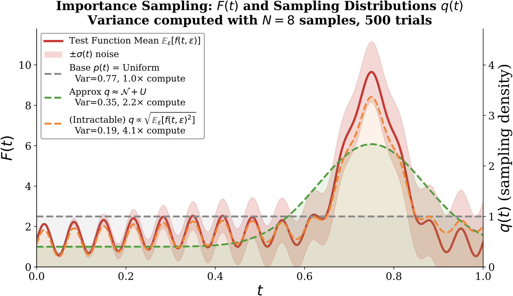
2. Timestep importance sampling: weight by where the gradient is
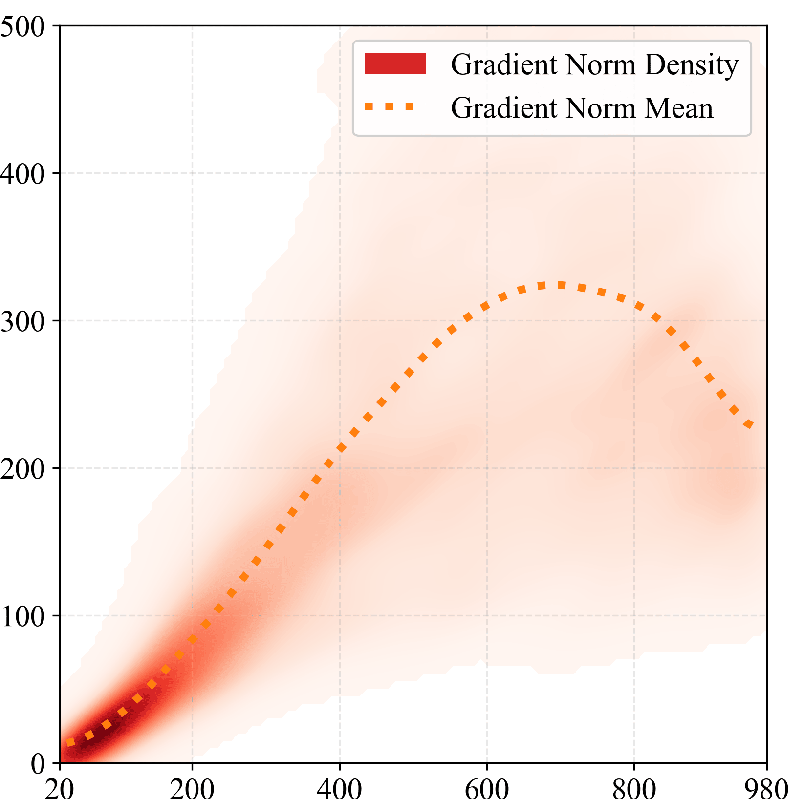
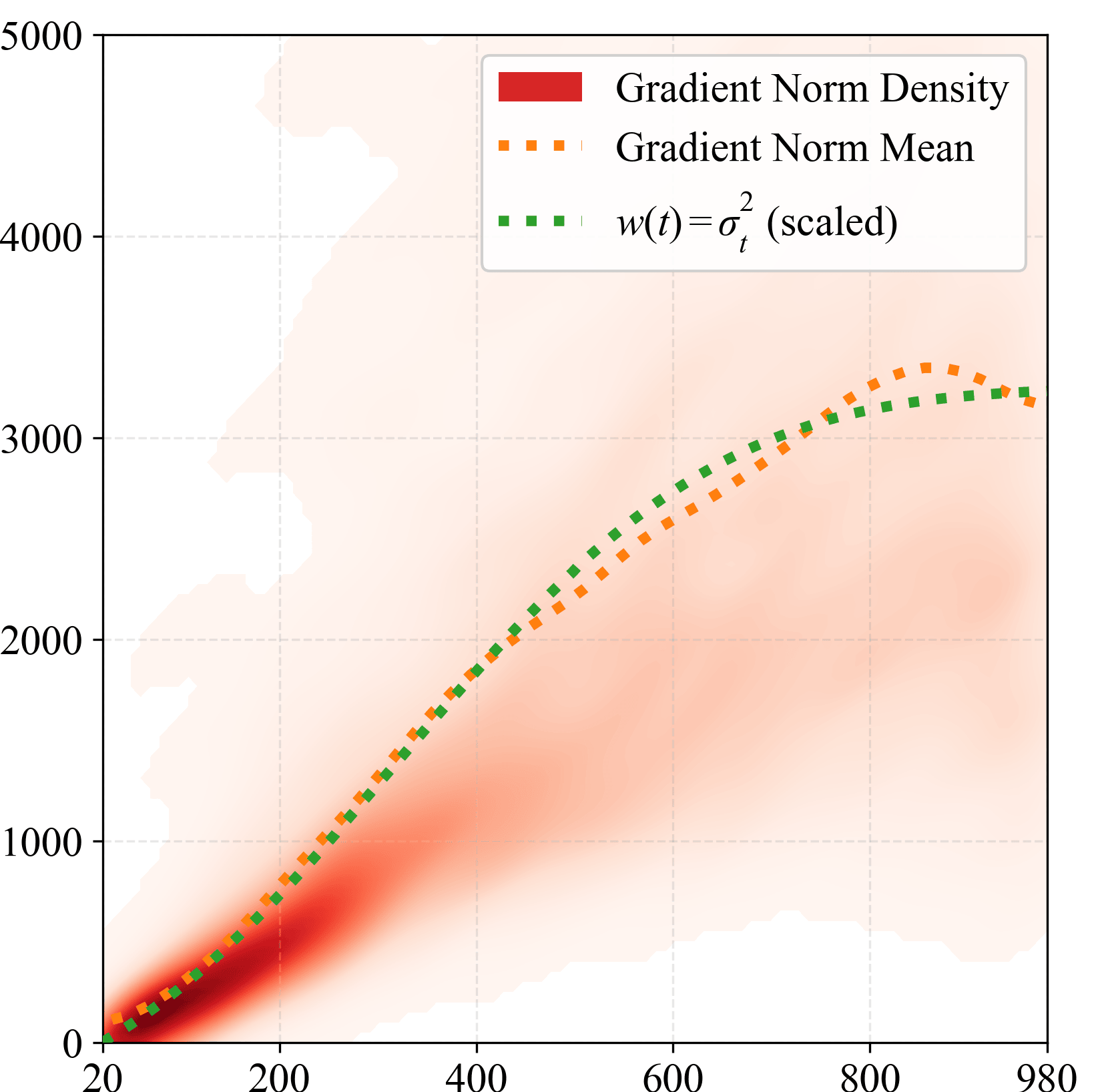
The variance-minimizing proposal is $q^\star(t) \propto p(t)\sqrt{\mathbb{E}[\,\|\mathbf{f}(t,\epsilon)\|^2 \mid t]}$. The renderer/encoder Jacobian reshapes timestep dependence: latent gradients peak mid-schedule, but parameter gradients we backpropagate track $w_{\mathrm{SDS}}(t)=\sigma_t^2$. So $w_{\mathrm{SDS}}$ is a free, accurate oracle surrogate.
Toy · oracle vs. surrogates
Sampled latent gradient norm
Timestep index $t$
Latent space · non-monotonic
Sampled parameter gradient norm
Timestep index $t$
Parameter space · tracks $w_{\mathrm{SDS}}(t)$
From toy to real data. Left: a toy illustration of the oracle importance proposal $q^\star(t) \propto p(t)\sqrt{\mathbb{E}[\|\mathbf{f}(t,\epsilon)\|^2 \mid t]}$, variance-equivalent to about $4\times$ uniform compute on this test function; a Gaussian-at-peak surrogate is worth ${\sim}2.2\times$. Middle: on real SDS runs the latent-space gradient norm is non-monotonic and peaks mid-schedule, so $w_{\mathrm{SDS}}$ alone is a poor proposal in latent space. Right: after backprop through the renderer and encoder, the parameter gradient is monotonic in $t$ and closely tracks $w_{\mathrm{SDS}}(t)=\sigma_t^2$ (dotted green), so $w_{\mathrm{SDS}}$ is a faithful zero-cost surrogate at the level we actually update.
3. Stratified inverse-CDF: spread your samples
Partition the timestep domain into $B$ bins, require one sample per bin, then map through the inverse-CDF of the importance-sampling proposal. Unbiased, never higher variance than IID at the same per-step cost, and stacks on top of step (2).
Stratified vs. IID samples
Inverse-CDF mapping to $q(t) \propto w_{\mathrm{SDS}}(t)$
Stratifying $u \in [0,1]$ guarantees one sample per bin; pushing through the inverse-CDF then maps those uniform draws into stratified samples from the importance-weighted proposal $q(t) \propto w_{\mathrm{SDS}}(t)$. Combines step (2) and step (3) without extra compute.
Results: effective compute multipliers
2.6 to 3.3×
SDS effective compute multiplier
Text-to-3D gradient variance, equal-cost baseline
2 to 3×
Data-attribution multiplier
Influence-score variance on Wan2.1 video attribution
10×
DMD gradient variance reduction
FID does not follow; see DMD section below
Text-to-3D distillation (SDS)
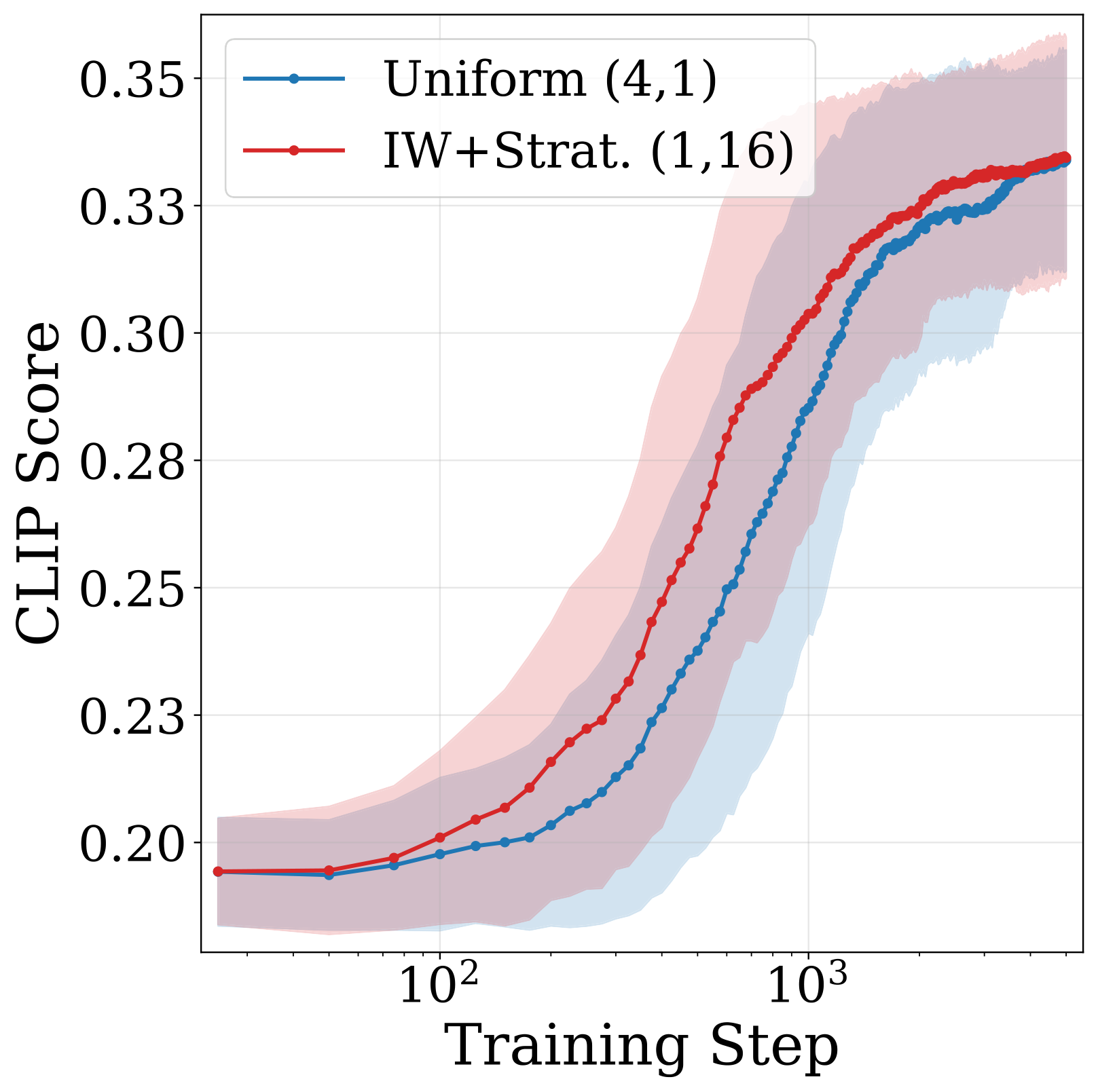
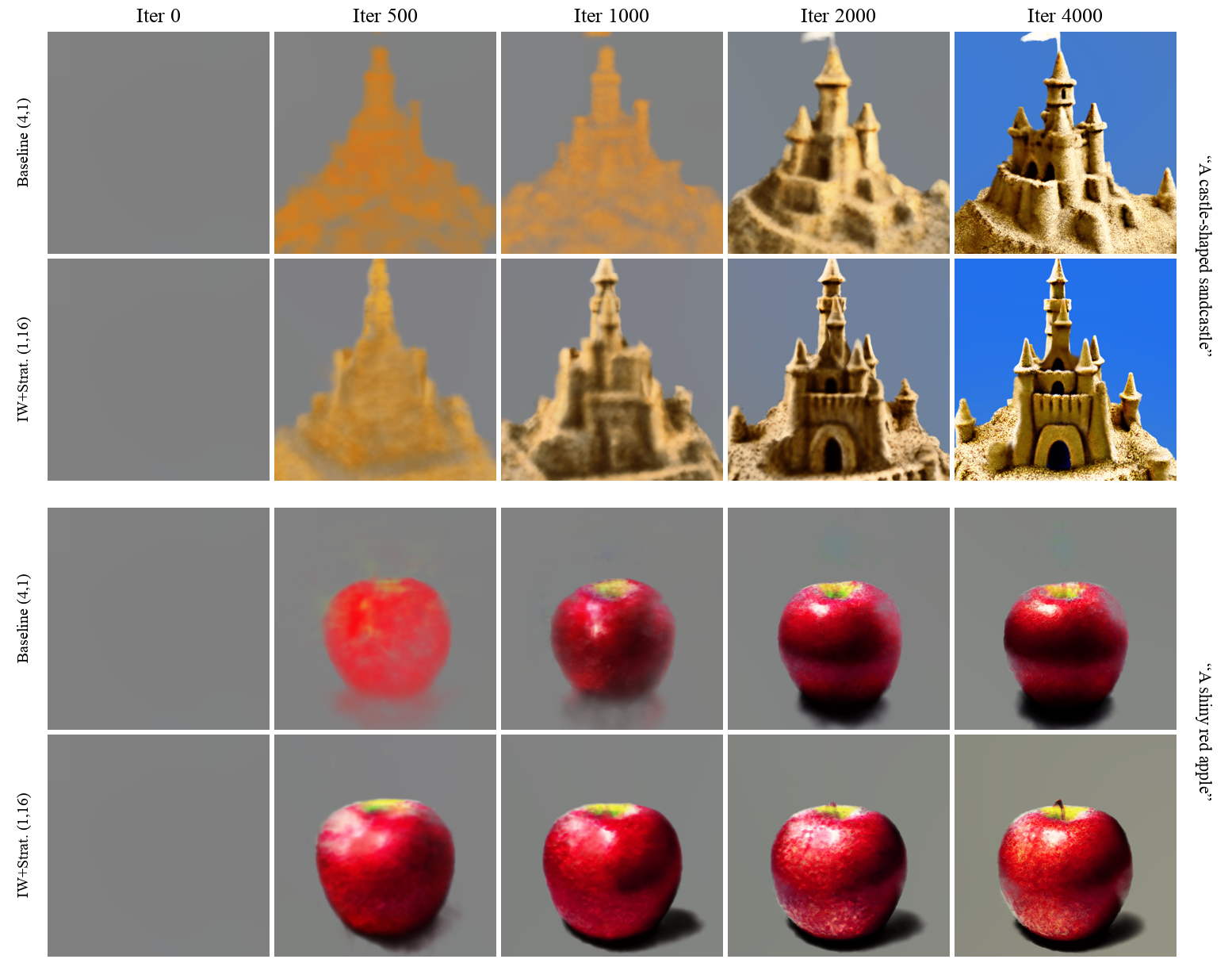
Three views of the same SDS sweep: CLIP score over training, qualitative renders along the same training axis, and the swept effective-compute frontier.
CLIP score · 30 prompts, 3 seeds, multi-view
Renders along the same training axis
Matched per-iteration cost (about 300-400 ms / iter). Top: CLIP score across training; CARV (red, IW+Strat, 1,16) sits above the uniform baseline (blue, 4,1) for the entire ramp before both saturate. Bottom: renders along the same iteration axis - CARV reaches near-converged geometry at $\sim$1k iterations while the baseline is still a coarse blob; both prompts show roughly $2\times$ wall-clock speedup to comparable quality.
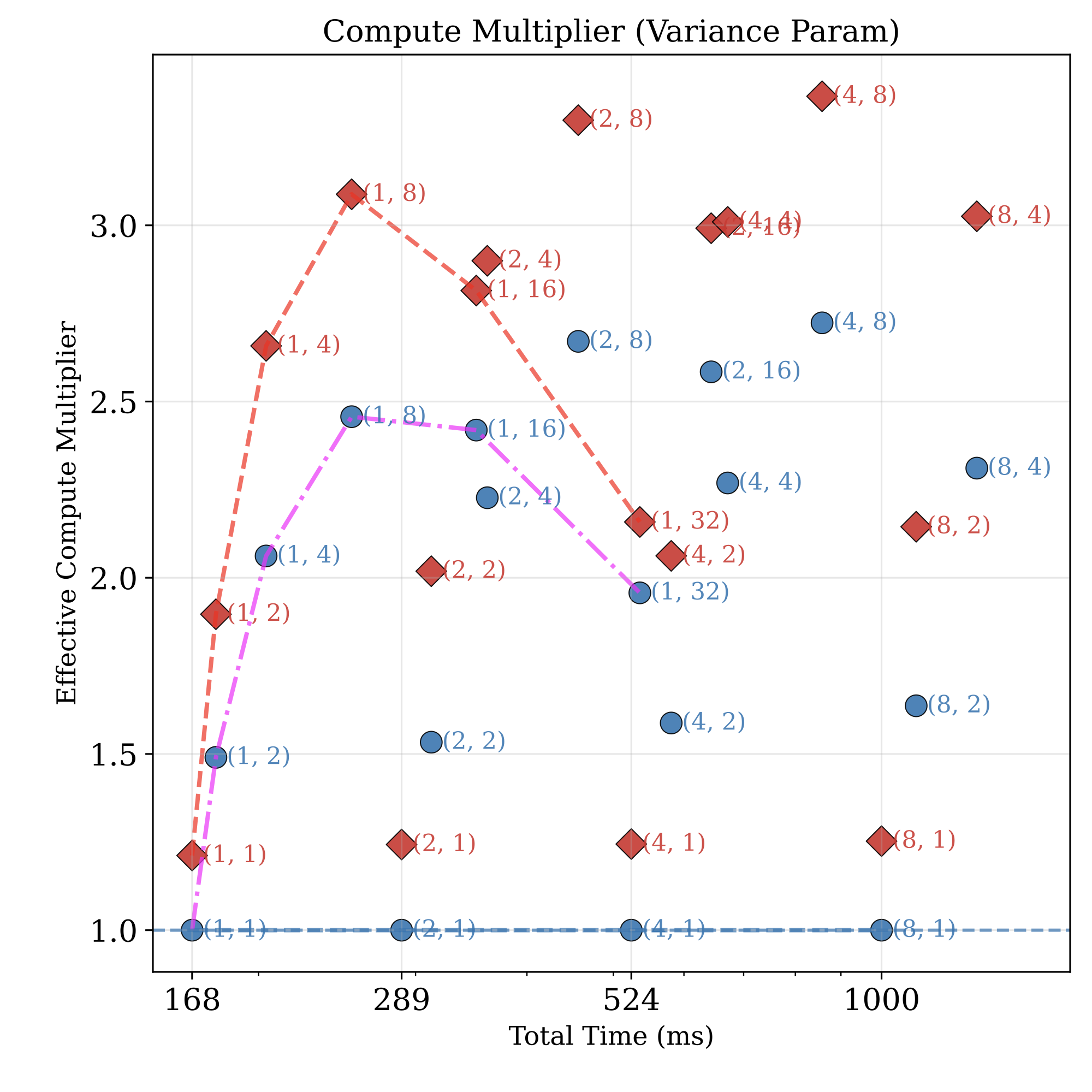
Effective compute multiplier (ECM) vs. equal-cost uniform baseline, swept over $(R, K)$ pairs at fixed total budget. The IW + stratified frontier (red) sits above uniform-only re-use (blue) at every compute point, peaking at 3.3× at $(R{=}4, K{=}8)$.
Each marker is a $(R, K)$ pair (renders, re-noisings); annotation shows the count. Red diamonds = IW + Stratified, blue circles = uniform. The dashed lines trace $(R{=}1, K)$ as $K$ grows. Hierarchical re-use drives most of the lift; IW + stratification add a free 20-25% margin on top.
Qualitative still renders
Final renders at the matched-budget end of the SDS runs. Baseline left, CARV right. Same prompts as the autoplay turntables above; these are the static frames at the end of training.
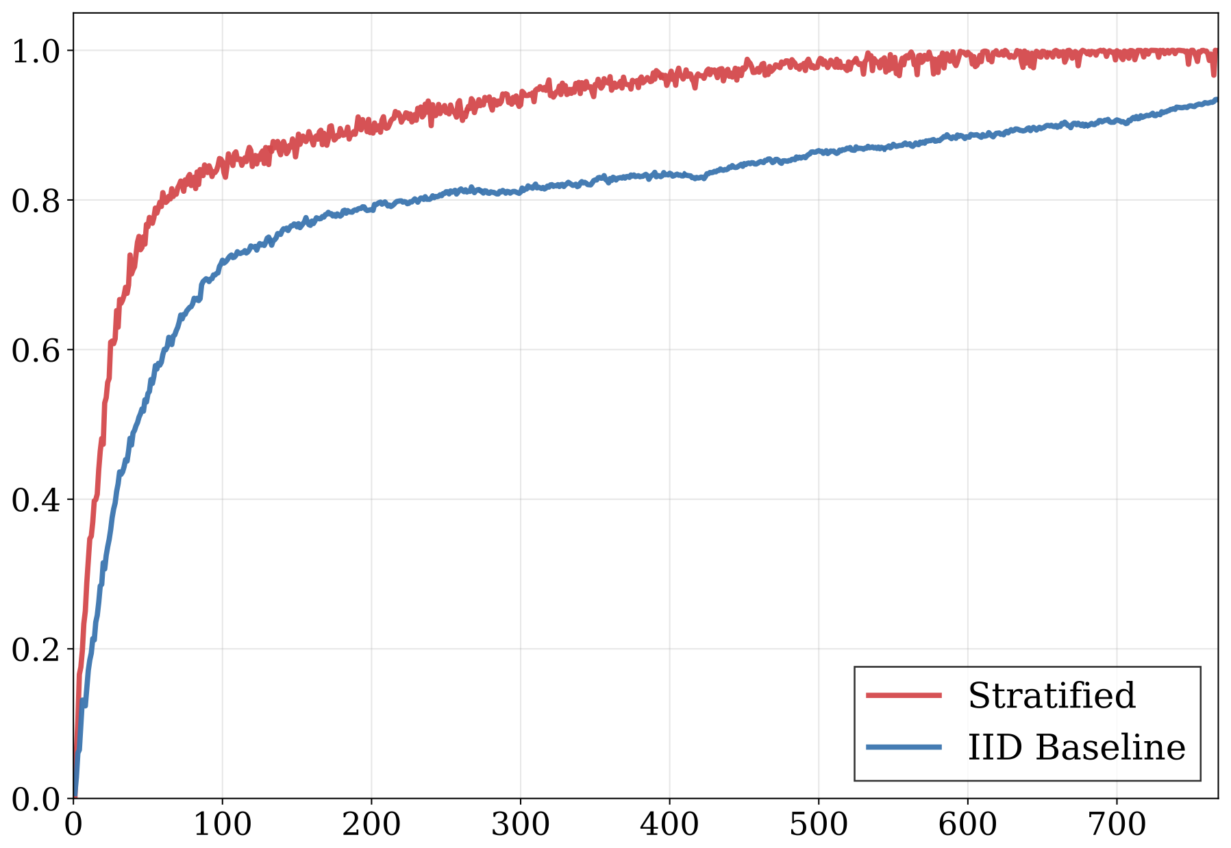
The same idea drops into MOTIVE-style video data attribution: gradient computations on Wan2.1-T2V become much cheaper to estimate accurately. Stratified sampling reaches the same correlation with ground-truth rankings using far fewer per-clip gradient samples than the IID baseline. Same 2 to 3 times multiplier story; full sweeps in the paper.
Mean Correlation
Gradient Samples per Data Point
Mean correlation of limited-sample influence rankings with ground-truth gradients on Wan2.1 video attribution (VIDGEN-1M, MOTIVE setup, leave-one-out over 11 queries). Stratified sampling (red) saturates near 1.0 well before the IID baseline (blue): a 1.3 to 3.8 times compute multiplier across budgets, over 2 times at practical budgets.
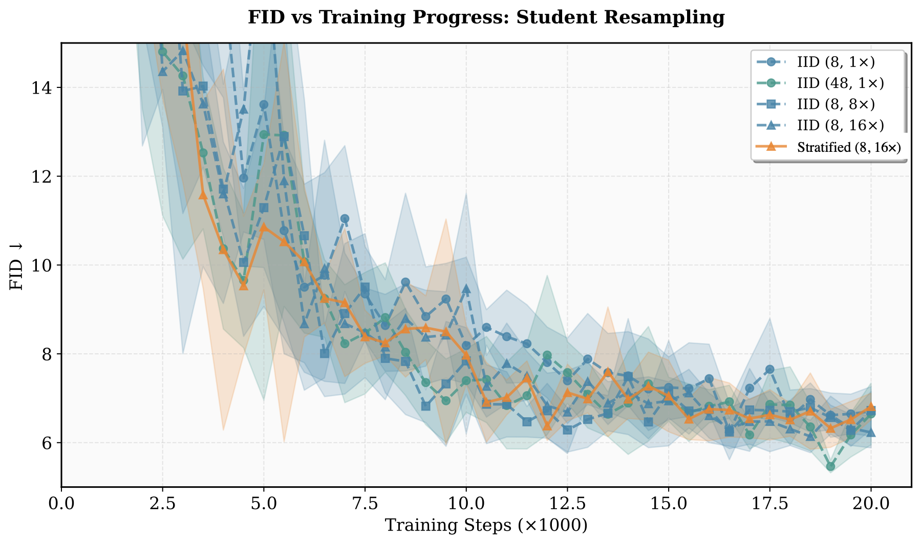
When MC variance is not the bottleneck: DMD
The same techniques cut DMD gradient variance by an order of magnitude, yet downstream FID barely moves. We treat this as a feature: DMD marks where MC variance stops being the bottleneck, and where the next gain must come from auxiliary stabilizers or input diversity.
Student FID across training. Stratified ($R{=}8$, $K{=}16$) cuts gradient variance by an order of magnitude over the matched IID setting (orange vs. blue dashed); FID stays inside the noise band of the IID curves. CARV is still unbiased and correct here, but lower variance does not unlock a better student in this regime.
When CARV helps, and when it does not
use it
Use CARV when…
The MC gradient (not its target) dominates wall-clock cost.
One render or encode is much more expensive than one diffusion noising step.
Pipelines: SDS (text-to-3D, audio-SDS, materials), data attribution (TRAK, MOTIVE), influence scoring, anything where rendering or encoding is the per-step cost.
caution
Be sceptical when…
Convergence is bottlenecked by other dynamics (auxiliary stabilizers, input diversity, optimizer state).
Render and denoise costs are comparable, so the multiplier collapses.
Pipelines: DMD-style single-step distillation, where 10 times variance reduction did not improve FID. CARV remains correct, but it does not reduce FID in this regime.
Takeaways
The framing
Diffusion-teacher gradients are Monte Carlo expectations.
Their variance per compute is the right axis to optimise, not raw step count.
The expensive randomness is the render or encode, not the noise.
Importance sampling: $q \propto p\,w_{\mathrm{SDS}}$, no extra compute.
Stratification: one sample per bin via inverse-CDF.
All three are unbiased and replace a few lines of code.
The limits
2 to 3 times ECM on SDS and attribution.
10 times variance reduction on DMD, but no FID gain.
Variance was the bottleneck on SDS, but not on DMD.
Citation
@misc{bettencourt2026carv,
  title={Variance Reduction for Expectations with Diffusion Teachers},
  author={Bettencourt, Jesse and Wu, Xindi and Atzmon, Matan and Lucas, James and Lorraine, Jonathan},
  year={2026},
  eprint={2605.21489},
  archivePrefix={arXiv},
  primaryClass={cs.LG},
  url={https://arxiv.org/abs/2605.21489},
}
Acknowledgements
We thank the Fundamental Generative AI Research (GenAIR) group at NVIDIA for the reference codebase and many helpful conversations during integration. We thank Sanja Fidler and the Spatial Intelligence Lab (SIL) for hosting the internship that made this collaboration possible. The text-to-3D experiments build on the open-source threestudio framework; the single-step distillation experiments build on the NVIDIA FastGen reference implementation.
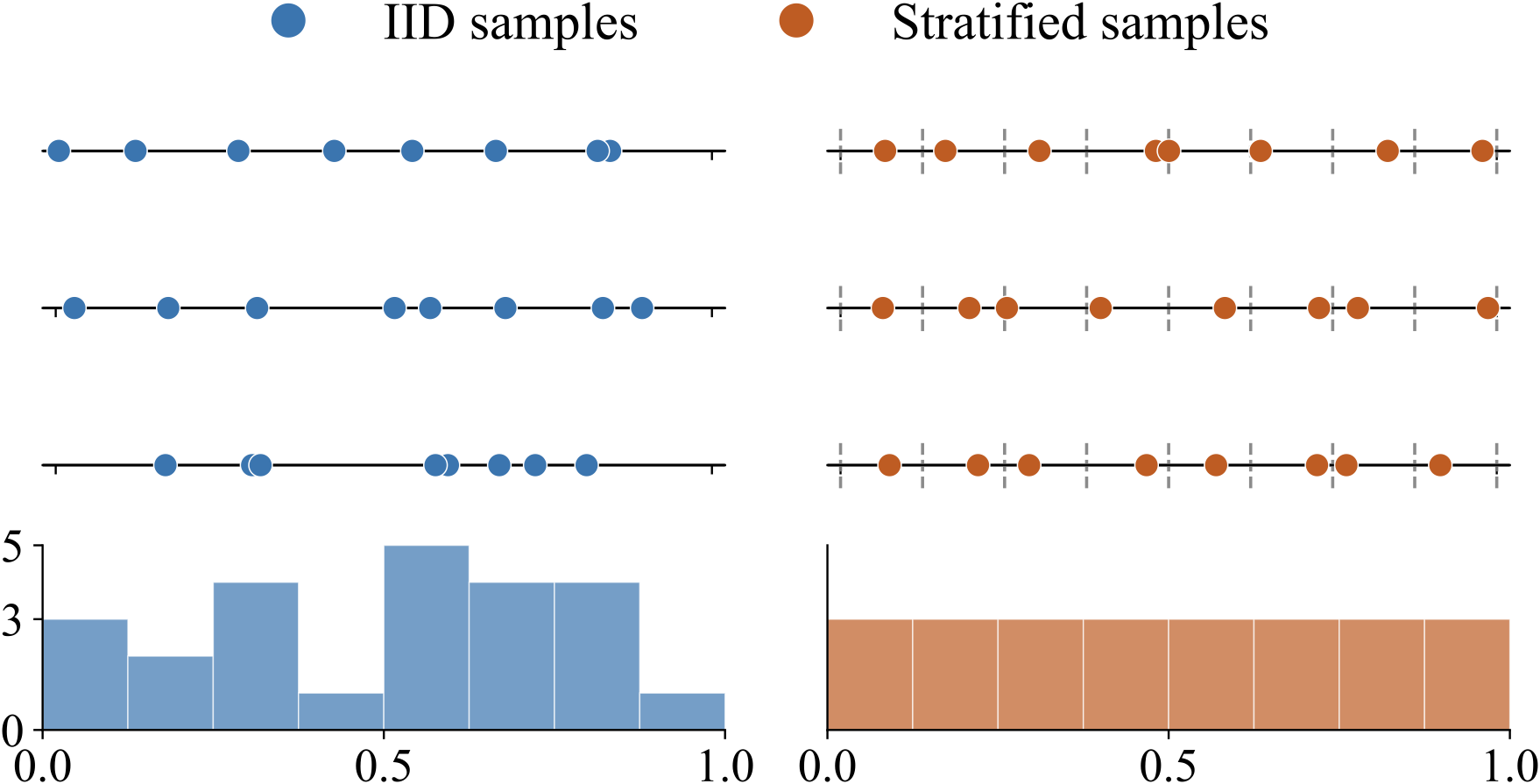
![Inverse-CDF construction: stratified u in [0,1] mapped through the CDF to non-uniform t samples that match the SDS importance weighting.](figures/stratified_inverse_cdf.png)