NVIDIAResearch
COMPASS

Ordered Clustered Routing at 100K Scale

Large delivery routes often visit clusters of stops, such as neighborhoods, in a prescribed order. COMPASS optimizes the paths inside all the clusters together with the bridges between them, by orchestrating parallel sub-solvers that are accelerated by reinforcement learning. It scales to 100,000 stops and works directly with road driving times.

Ido Greenberg, Hugo Linsenmaier, Piotr Sielski, Shie Mannor, Alex Fender, Gal Chechik, Eli Meirom
NVIDIA
arXiv preprint, 2026
COMPASS in three minutes.

Abstract

Large-scale routing often requires visiting clusters of nodes in a prescribed order, giving rise to the Ordered Clustered Traveling Salesman Problem (OCTSP). Optimizing each cluster independently seems natural, but misses non-local dependencies. We introduce the COMPASS algorithm for OCTSP, which combines search with learning-accelerated routing by orchestrating parallel sub-solvers. COMPASS has no quality ceiling and its solutions keep improving with compute. It exploits the clustered structure, and can reach exact solutions in time exponential in cluster size rather than instance size. Empirically, COMPASS consistently outperforms alternative methods. Unlike common large-scale routing solvers, COMPASS consumes general distance matrices and is not limited to coordinate inputs. We demonstrate scaling to 100K synthetic nodes and to 28.5K real e-commerce nodes. To our knowledge, the latter is the largest reported routing solution over asymmetric distances, 9x beyond established ATSP benchmarks.

The problem

In the Ordered Clustered Traveling Salesman Problem, locations are grouped into clusters with a fixed order, and all the locations of one cluster must be visited before those of the next. This arises, for example, in last-mile delivery with time slots, where each neighborhood is served before the next one.
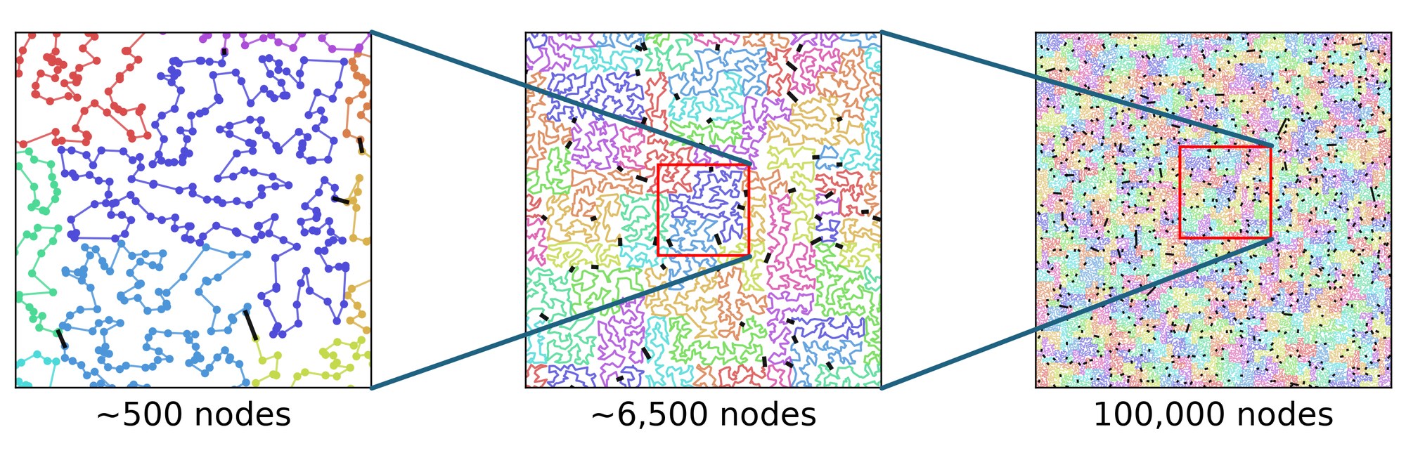
A route through 100,000 nodes shown at three zoom levels: about 500 nodes, about 6,500 nodes and all 100,000 nodes. Clusters are drawn in different colors and are connected by short black bridges.
A COMPASS solution with 100,000 nodes at three zoom levels. Clusters (in colors) must be visited in a prescribed order; bridges (in black) connect the clusters at locations chosen by the solver.

Solving each cluster on its own and then connecting the clusters is natural, but can be far from optimal. The path through a cluster depends on where it enters and exits the cluster, and these endpoints determine the cost of the bridges to the adjacent clusters. The dependence is also global: a change in one cluster can change the best path in a distant one.
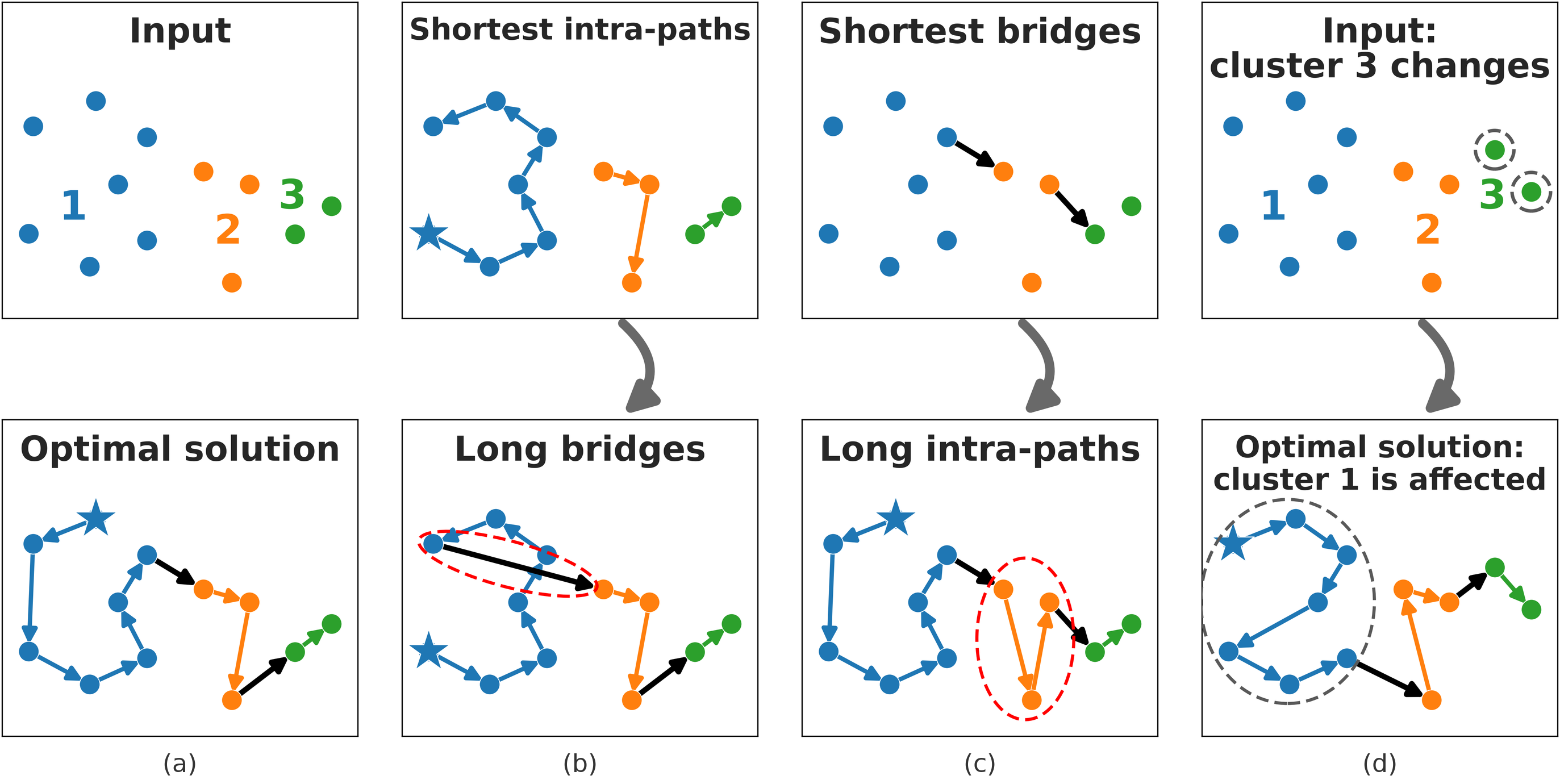
Four toy examples with three clusters. (a) The input and its optimal solution. (b) The shortest paths inside the clusters lead to long bridges. (c) The shortest bridges lead to long paths inside the clusters. (d) A change in cluster 3 changes the optimal path in cluster 1.
(a) A toy problem and its optimal solution. (b) Committing to the shortest paths inside the clusters forces a long bridge. (c) Committing to the shortest bridges forces long paths. (d) Changing cluster 3 changes the optimal path in cluster 1.

Method

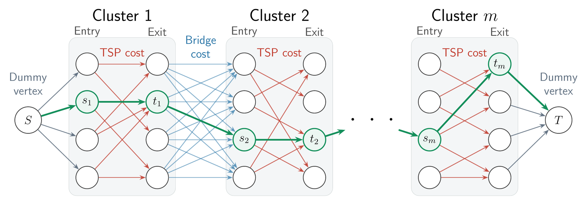
COMPASS represents the whole chain of clusters as one directed graph. For every cluster it selects candidate pairs of entry and exit nodes, and each pair defines a small routing problem with fixed endpoints. These sub-problems are solved in parallel on GPUs, by a solver accelerated with reinforcement learning (EARLI) whose neural network reads raw distance matrices, so it applies to asymmetric road distances and not only to coordinates. Bridges connect each exit to the entries of the next cluster, and the shortest path through the graph gives the complete route.

The COMPASS graph: every cluster has a column of entry nodes and a column of exit nodes. Red edges from entries to exits carry the cost of the route inside the cluster, blue edges from exits to the entries of the next cluster carry bridge costs, and the shortest path from the start vertex to the end vertex is marked in green.
Red edges are routes inside a cluster between a candidate entry and exit; blue edges are bridges. The shortest path (green) is the solution.

Because all the clusters are modeled together, COMPASS has no quality ceiling: with more compute and more time its solutions keep improving, and it can reach exact solutions in time exponential in the cluster size rather than the instance size.

Results

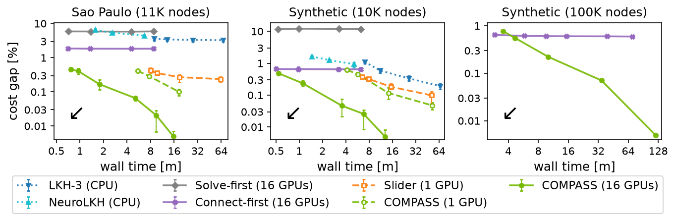
On real e-commerce orders in São Paulo with 11,000 stops and road driving times, COMPASS reaches a cost gap of 0.46% from the best known solution within 0.7 minutes. The earlier large-scale solvers LKH-3 and NeuroLKH reach gaps of 3.11% after 67.8 minutes and 4.29% after 6.8 minutes.

Cost gap against wall time on Sao Paulo with 11K nodes, synthetic data with 10K nodes and synthetic data with 100K nodes. The COMPASS curves are the lowest at every time budget and keep decreasing.
Cost gap against optimization wall time (lower is better). Solve-first, Connect-first and Slider are baselines introduced in the paper.
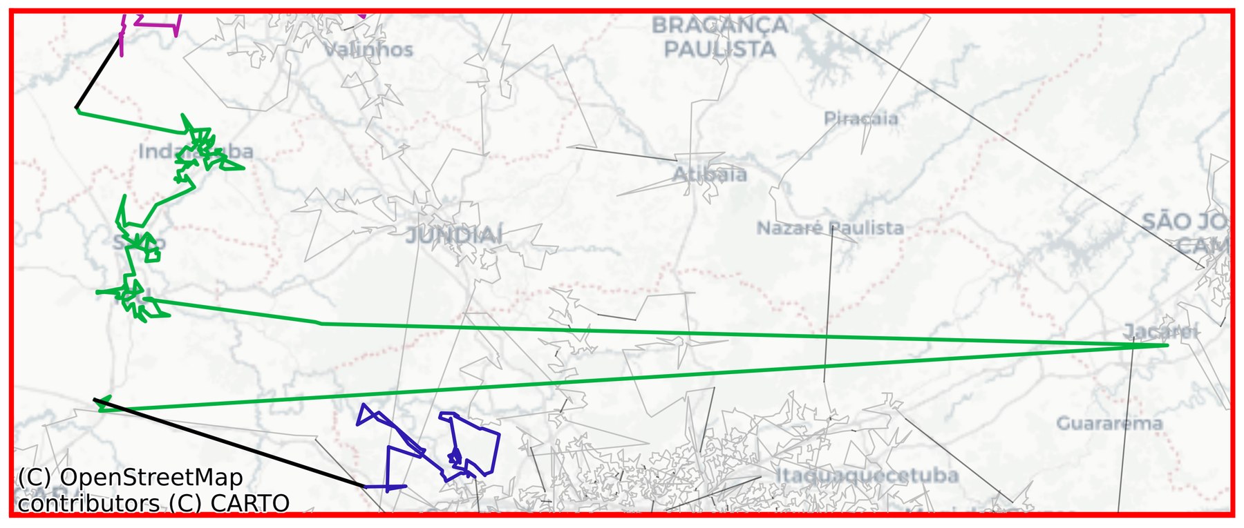
Part of a Sao Paulo solution of the Connect-first baseline: a short bridge between two clusters is followed by a very long edge inside a cluster.
Connect-first chooses the shortest bridges (black), which leads to very long edges inside a cluster (green).
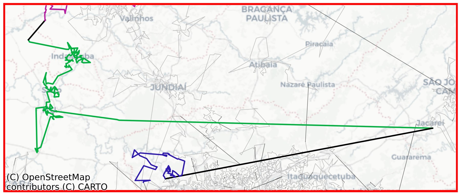
The same part of the Sao Paulo solution of COMPASS: a longer bridge between the clusters avoids the long edge inside the cluster.
COMPASS chooses a longer bridge and avoids the long edges, which lowers the total cost.

Edges are drawn as straight lines for display; costs are road driving times. Map data © OpenStreetMap contributors © CARTO.

BibTeX

@article{greenberg2026compass,
  title   = {COMPASS: Ordered Clustered Routing at 100K Scale},
  author  = {Greenberg, Ido and Linsenmaier, Hugo and Sielski, Piotr and Mannor, Shie and Fender, Alex and Chechik, Gal and Meirom, Eli},
  journal = {arXiv preprint arXiv:2609.20352},
  year    = {2026}
}