Cluster Search#

Search mode: query-free browsing of precomputed groups of similar clips.

Cluster search browses precomputed groups of visually and semantically similar clips, ranked by proximity to the cluster centre. Unlike every other search mode, it requires no query: clusters surface the natural structure of the dataset, revealing recurring scenarios and edge cases that you would not know to search for. It is the fastest way to get an overview of what a new dataset contains.

Reach for it when you do not yet know what to look for: surveying what scenarios a new dataset actually holds, spotting near-duplicates, seeding hard examples from the sparse edges of a cluster, or checking that every scenario you expect is represented. See Common Patterns for the detailed cases.

Reach for something else when you already know what you are after. Every other search mode takes a query and will get there directly.

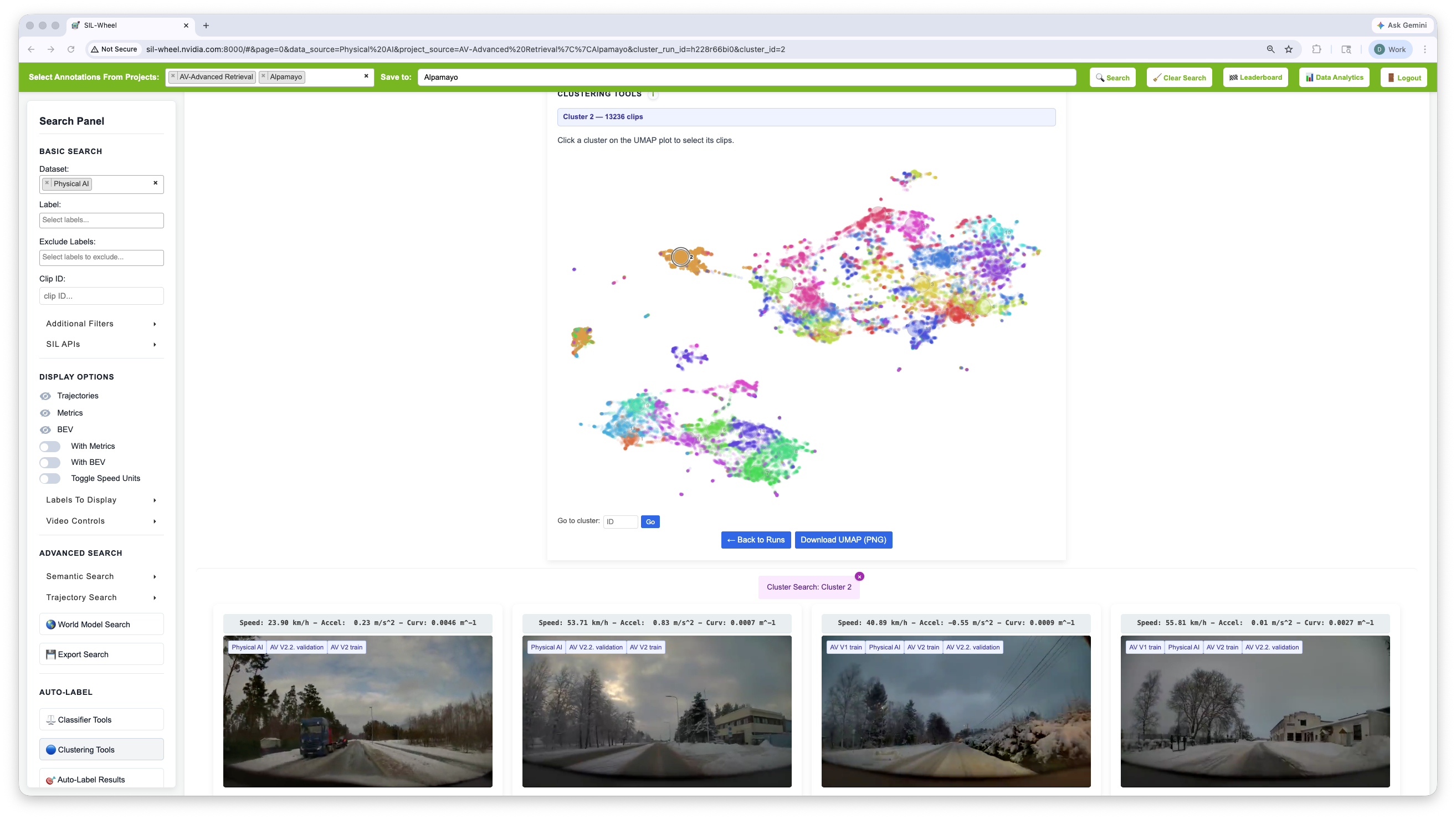
A UMAP scatter of colour-coded clusters with one cluster selected, and its member clips listed below — Browsing Cluster 2: 13,236 visually similar snow-covered road clips, ranked by distance to the cluster centroid.#

How It Works#

Clustering groups clips by running k-means over their precomputed embeddings. Within a cluster, clips are ranked by distance to the centroid: the most representative examples appear first, more peripheral ones later. A UMAP projection of the embedding space is shown alongside the cluster list, giving a visual overview of how clusters relate to each other.

Clusters are not labelled automatically. Part of the value of this mode is discovering structure in the data without specifying what to look for. A cluster might contain all clips from a particular intersection type, weather condition, or driving behaviour without any of those concepts having been searched for explicitly.

The clustering panel is built around three views, navigated through a breadcrumb at the top of the panel (Run › Cluster › Range):

Run overview – the full UMAP scatter, every cluster shown.
Cluster selection – one or more clusters highlighted; results grid filtered to the corresponding clips.
Zoomed (beeswarm) view – a single cluster expanded so each member clip is laid out by its distance to the centroid.

Clicking a higher-level segment in the breadcrumb (e.g. the run name) collapses back to that level without losing the selected run.

Running Clustering#

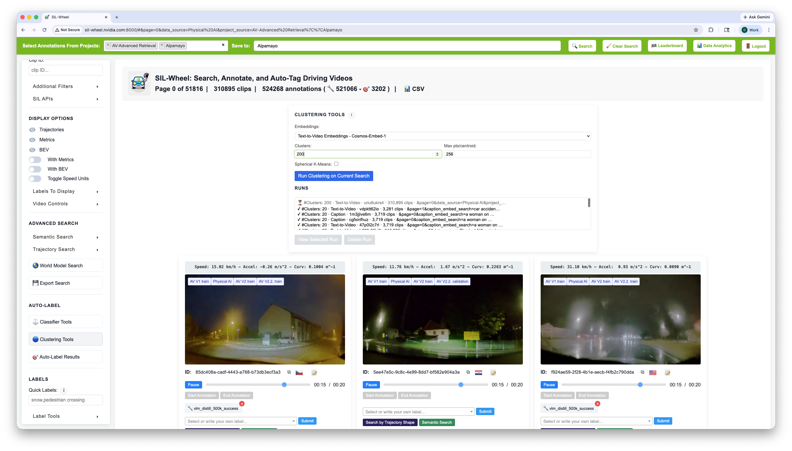
The Clustering Tools panel with embedding type, cluster count and max points per centroid set, above a list of previous runs — The clustering configuration panel. Runs are listed with their status, cluster count, embedding type, and the number of clips they cover.#

Clustering is launched from the Clustering Tools panel and each run is configured with the following parameters:

Two settings matter:

Number of clusters sets the granularity. A small number surfaces broad scenario categories; a large one (up to 20 000) reveals variation within them. Runs at different counts coexist, so the same data can be explored at several levels of detail.

Embedding type decides what “similar” means. The three spaces are the same ones behind Semantic Search, Caption Embedding Search, and Visual Search: video content, caption text, and frame appearance respectively. Video content is the default and the right choice for discovering scenario types.

Spherical k-means and max points per centroid are tuning knobs; the defaults suit most datasets.

A run is scoped to the search that was active when it launched, so filtering first clusters only that slice. Runs execute in the background, three at a time, and become browsable the moment they finish.

Clustering Offline at Scale#

The in-UI launcher is the right path for runs of up to a few hundred thousand clips. Beyond that, k-means and UMAP are better run outside the server, somewhere the embedding files can be read locally: the same machine the server sits on may not have spare GPU/CPU for a multi-million-clip k-means, and queuing it through the server ties up one of the three concurrent slots for the duration. Offline clustering also lets you tweak k-means and UMAP knobs that the in-UI panel does not expose (--n-iter, --n-redo, --seed, --umap-n-neighbors, --umap-min-dist).

Wheel ships an example script, examples/cluster_from_search.py, that automates the round trip:

Build the search you want to cluster in the browser and copy the URL.
Run the script with that URL plus a path to the embeddings directory. It pulls the matching clip IDs over HTTP, reconstructs their embeddings from the local FAISS index, runs k-means and UMAP, and (optionally) extracts caption topics.
The script then calls POST /upload_clustering to ship the run directory back to the server. After the upload the run shows up in the Clustering Tools panel exactly like an in-UI run, with the same UMAP, beeswarm, and Top clusters for… views available.

The same upload endpoint is also exposed as WheelHTTPClient.upload_clustering_run for callers that already build their own clustering runs and only need to register them with the server. --embed-type other is supported when the vectors come from an external model: clustering and UMAP still work, but the Top clusters for… text query is disabled because the server has no encoder registered for that type.

Exploring a Run#

A completed run is browsed through a 2-D UMAP projection where spatial proximity reflects embedding similarity. Centroids are sized by membership; hovering one previews its representative clip, clicking selects it, and dragging a box selects every cluster inside.

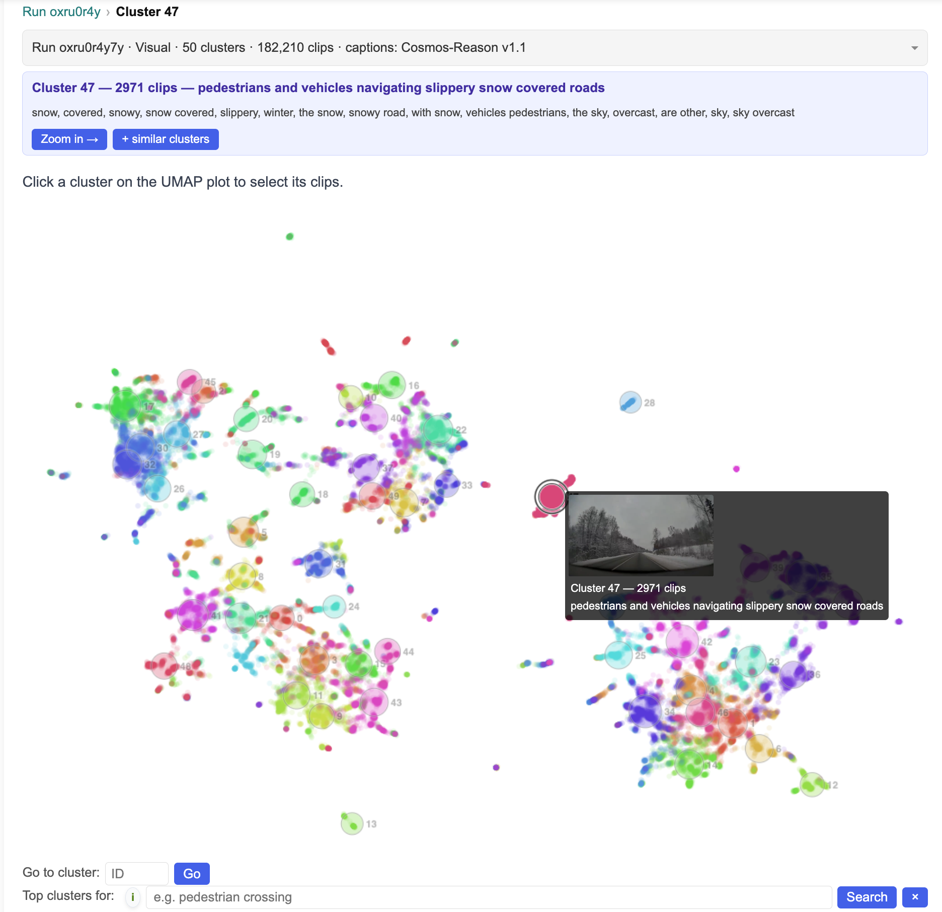
A UMAP scatter of 50 numbered cluster centroids with one hovered, showing a clip thumbnail and the cluster topic summary — Run overview: centroids sized by membership count, click to select, drag to box-select multiple clusters at once.#

Selecting a cluster also unlocks + similar clusters, which pulls in the five nearest clusters in UMAP space. That is the quickest way to widen from one scenario to a neighbourhood of related ones.

Zooming into a single cluster replaces the scatter with a beeswarm: each member clip is a dot placed by its distance to the centroid, graded blue (close) to orange (far).

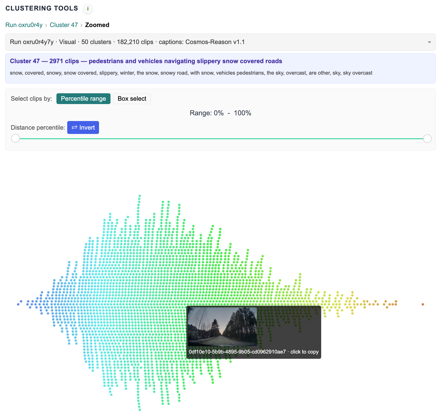
A beeswarm of the clips in one cluster, colour-graded blue to orange by distance from the centroid, with a hovered clip thumbnail — Zoomed beeswarm: each member clip is a dot positioned by its distance to the centroid.#

Selecting Clips by Distance#

Distance to the centroid is the useful axis inside a cluster: the closest clips are the most representative, the furthest are the edge cases. Two modes narrow the results to a band of it.

Percentile range is a slider over the distance distribution. 0–10% keeps the most representative clips, 90–100% keeps the periphery, and ⇄ Invert flips between the two.

Box select drags the same band directly on the beeswarm, which is more precise when the distance distribution is uneven.

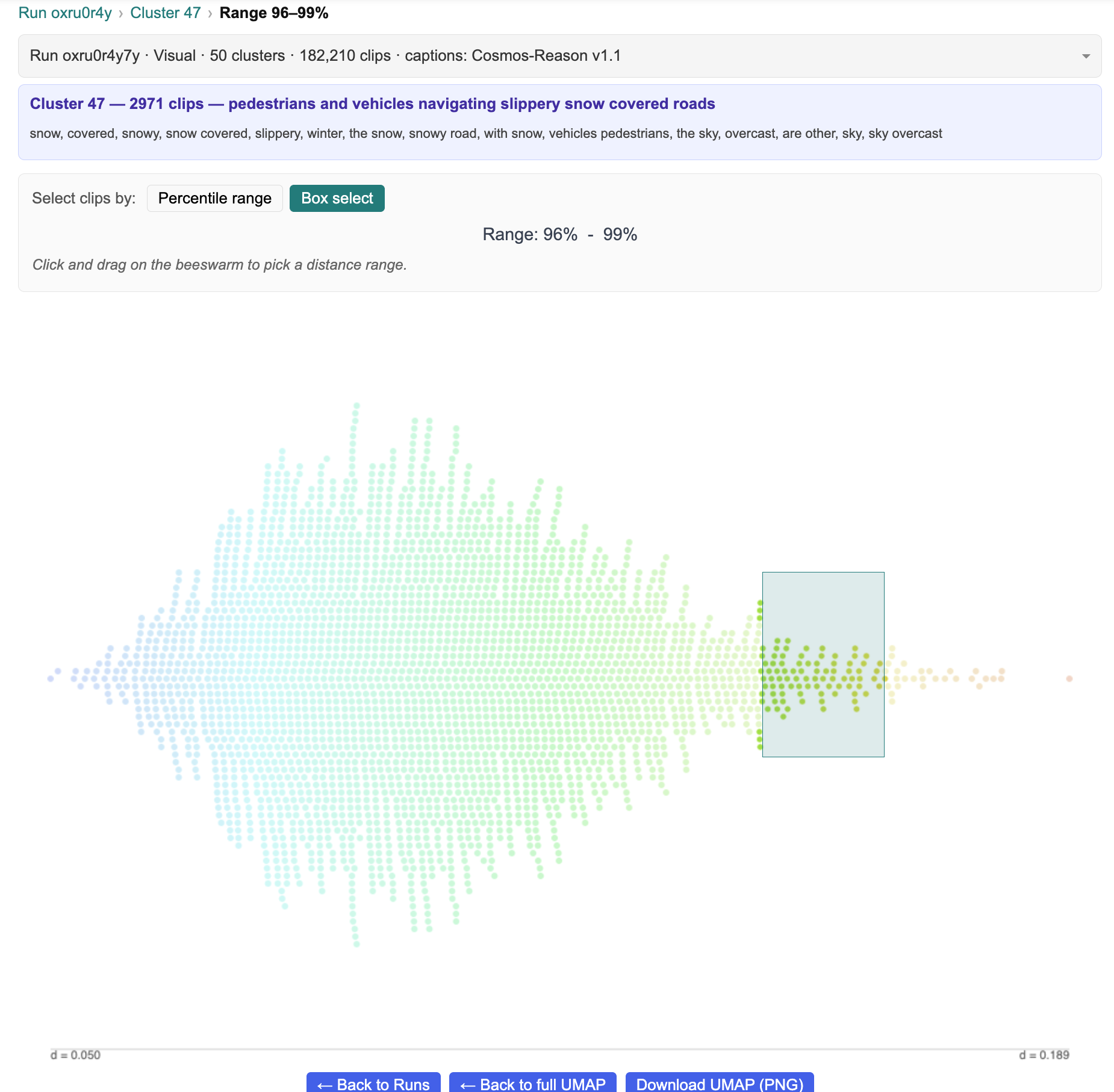
The beeswarm in Box select mode with a drag rectangle over the right tail, selecting the 96 to 99 percent distance range — Selecting clips by dragging a rectangle across the beeswarm. The Percentile range mode makes the same selection through a slider.#

Finding Clusters by Text#

On a run with hundreds of clusters, Top clusters for… jumps straight to the ones worth opening. It matches a text query against the centroids and returns the closest ten, each with its size, distance, and topic keywords. The query is encoded with the same model that built the run, so “closest” means the same thing here as it does in the clustering itself.

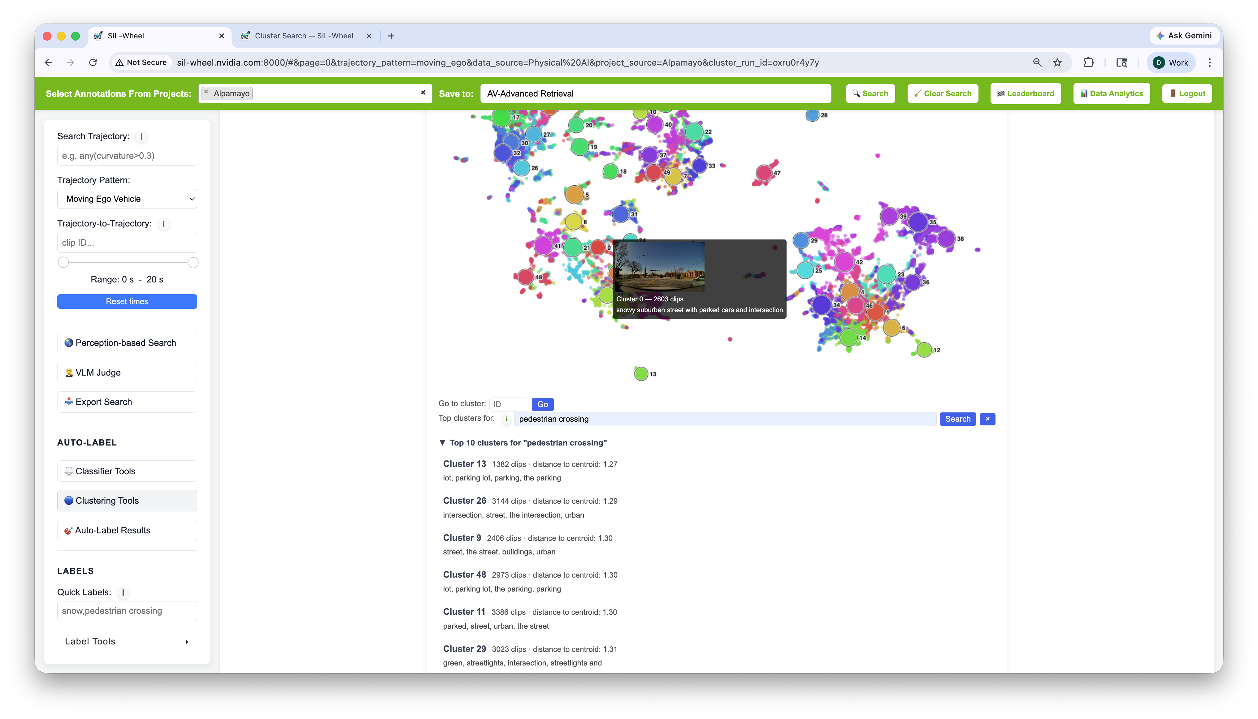
A ranked list of the top ten clusters for the query pedestrian crossing, each with its clip count, centroid distance and keywords — Searching for the top clusters matching a text query within a clustering run.#

Topic Modeling#

Each cluster is automatically labelled with keywords drawn from the captions of its member clips, plus a short LLM-generated description. The labels make it possible to scan a clustering run at a glance, without watching every representative video, and decide which clusters are worth opening.

Keywords are extracted by TF-IDF over a sample of each cluster’s captions, filtered against generic driving terms, and the top 15 are kept. Extraction runs automatically as part of the clustering job. The keywords and description appear in the cluster panel and in the UMAP hover tooltip.

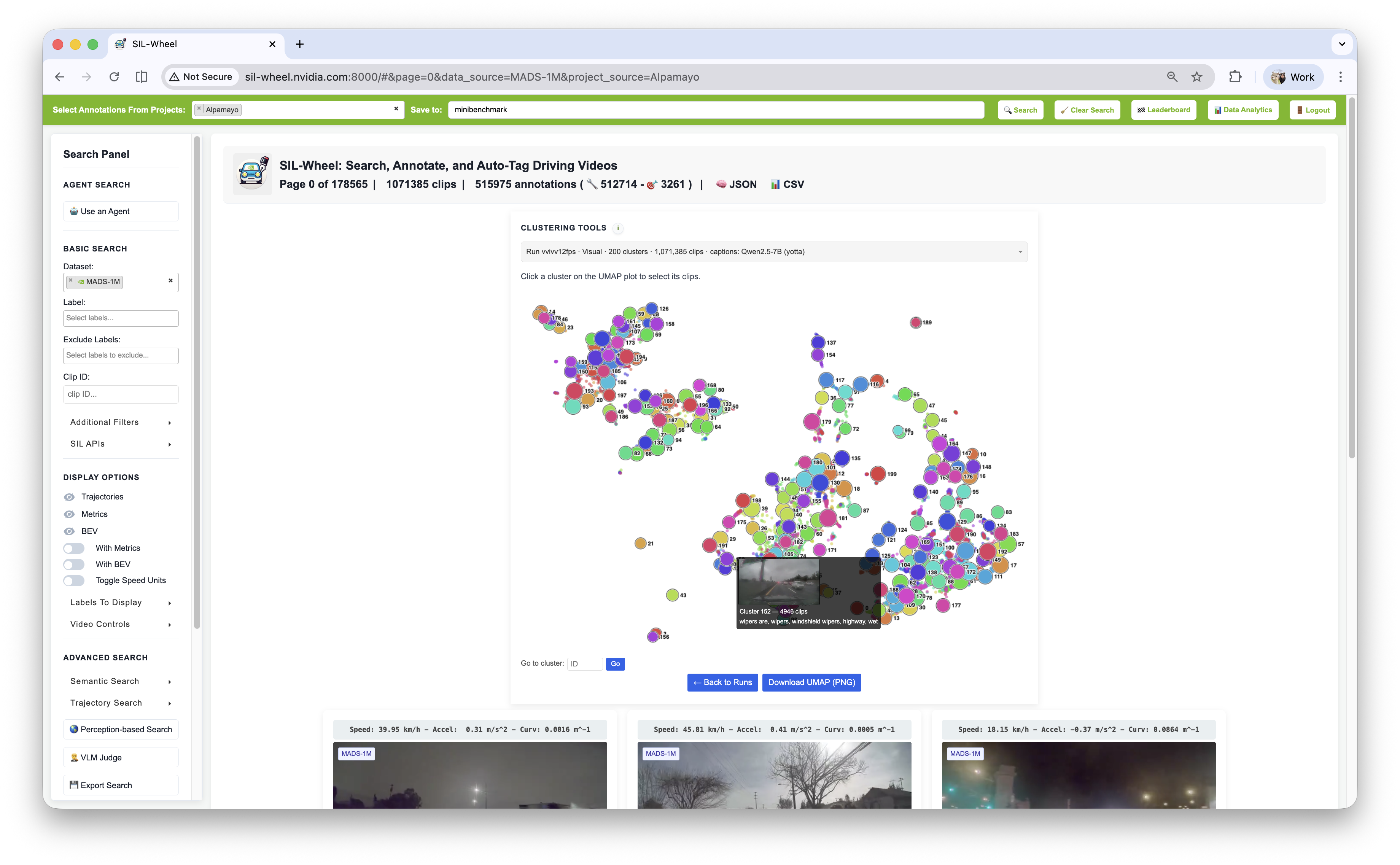
A UMAP of 200 clusters with one hovered, its tooltip listing the clip count and the topic keywords wipers, windshield wipers, highway, wet — Hovering a cluster surfaces its topic keywords and clip count; the run details appear above the plot.#

Topics need a captions database (--captions_db); without one, clusters are labelled by ID and size alone. Descriptions additionally need the configured LLM provider’s credentials, and are skipped silently if absent.

Common Patterns#

Cluster search is most useful for:

Data exploration: understanding what scenarios are common or rare in a dataset before deciding what to annotate or evaluate.
Deduplication review: a cluster of very similar clips often signals near-duplicates in the dataset, which can then be curated or down-sampled.
Hard-example seeding: browsing cluster peripheries surfaces clips that do not fit neatly into any group, often the most challenging and informative edge cases.
Distribution validation: checking that all desired scenario types are represented in the dataset by verifying that meaningful clusters exist for each of them. Sparse or absent clusters signal gaps in coverage that may need to be filled before training or evaluation.

Cluster Search

Contents